Cheatsheet: Soil Mechanics

1. Soil Classification and Properties

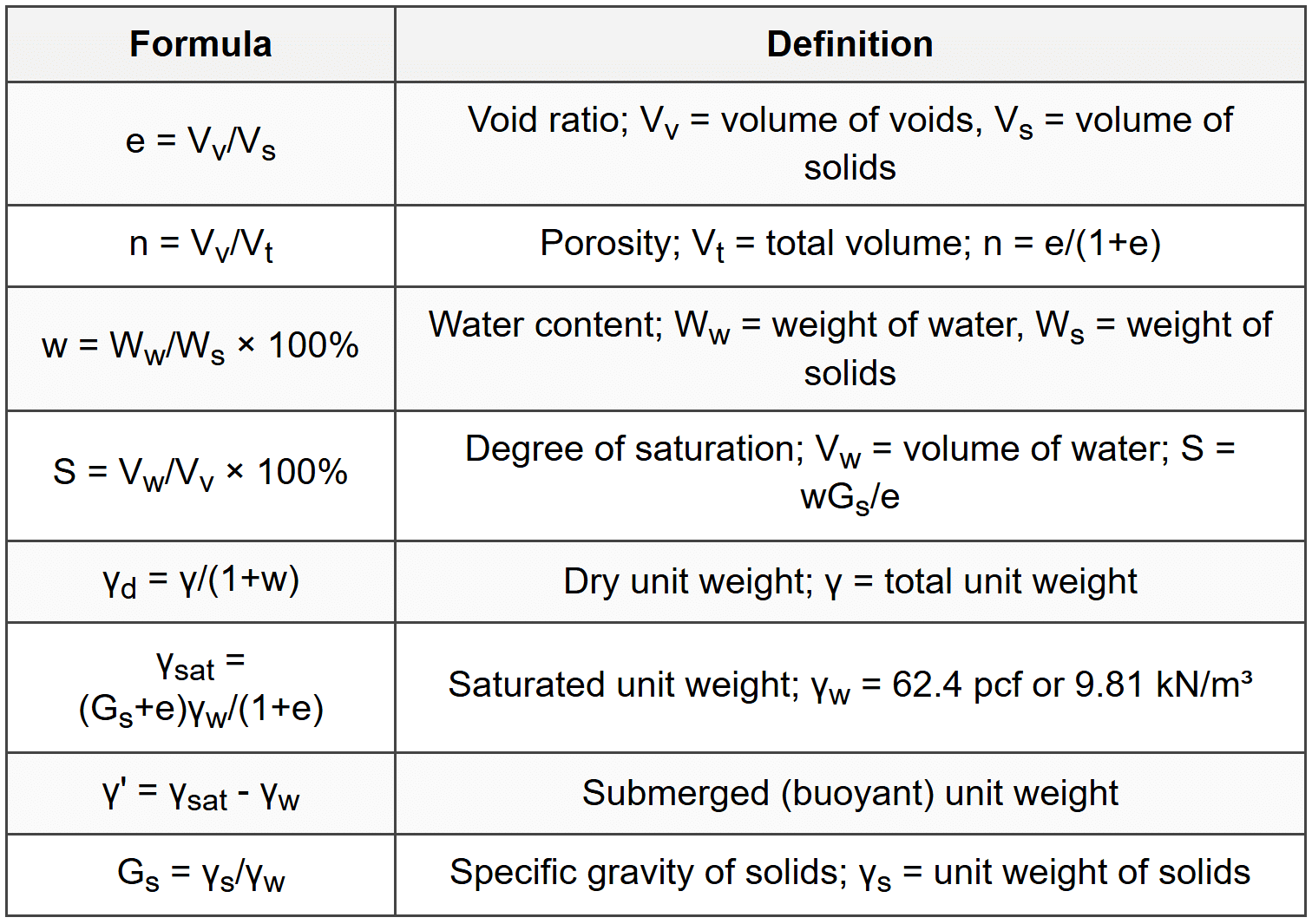
1.1 Phase Relationships

1.2 USCS Classification

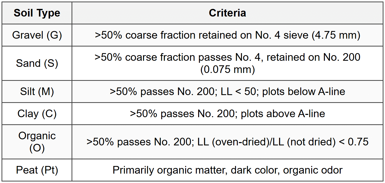
1.2.1 Coarse-Grained Soil Symbols

• W = well-graded; C_u ≥ 4 (gravel) or ≥ 6 (sand) AND 1 ≤ C_c ≤ 3
• P = poorly graded; does not meet well-graded criteria
• M = contains fines with low plasticity (plots below A-line)
• C = contains fines with high plasticity (plots above A-line)
• If 5-12% fines: dual symbol (e.g., GW-GM)
• If >12% fines: classify by fines (e.g., GM, GC)

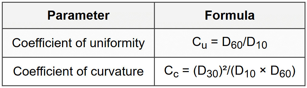
1.2.2 Gradation Coefficients

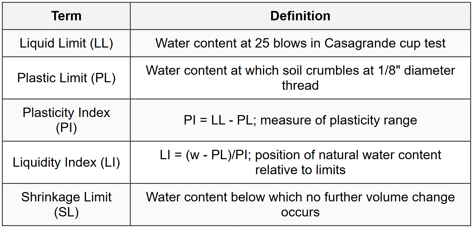
1.3 Atterberg Limits

1.3.1 Plasticity Chart (A-Line)

• A-line equation: PI = 0.73(LL - 20)
• Above A-line: Clay (C); Below A-line: Silt (M)
• LL < 50: Low plasticity (L); LL ≥ 50: High plasticity (H)
• CL-ML: plots in hatched zone between PI = 4 and A-line

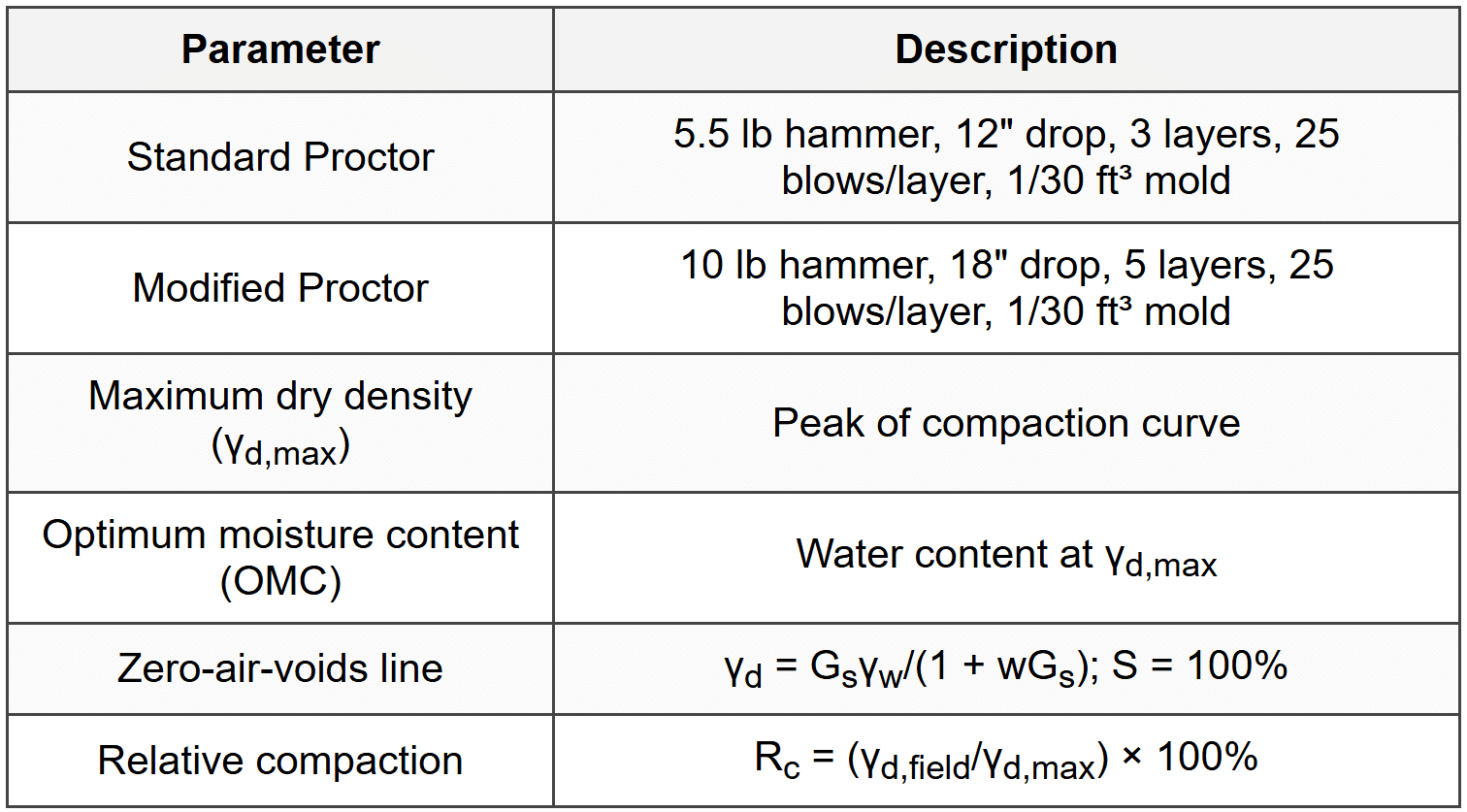
1.4 Soil Compaction

1.5 Relative Density

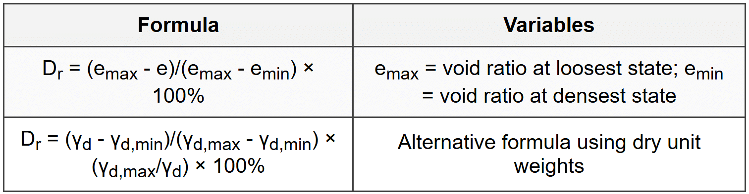
• D_r < 15%: Very loose; 15-35%: Loose; 35-65%: Medium; 65-85%: Dense; >85%: Very dense

2. Hydraulic Properties and Flow

2.1 Darcy's Law

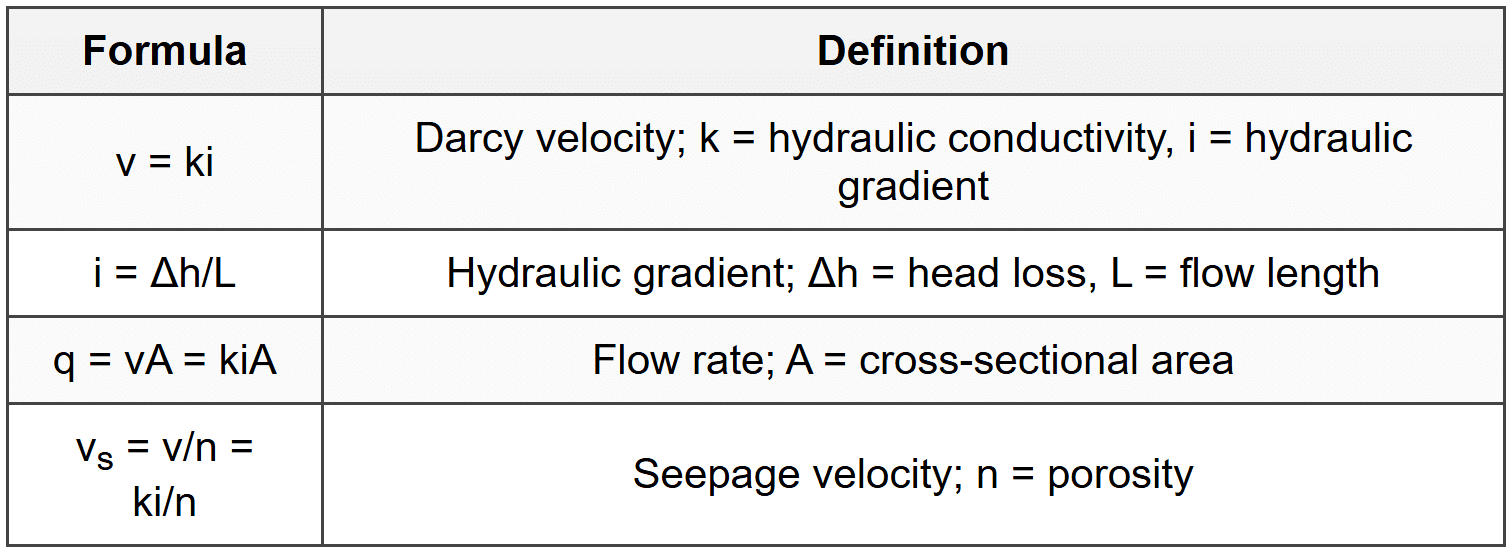
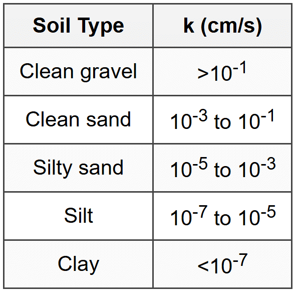
2.2 Hydraulic Conductivity

2.2.1 Empirical Formulas

• Hazen: k (cm/s) = C(D₁₀)² where C = 100-150, D₁₀ in cm; valid for 0.1 mm < D₁₀ < 3 mm
• Temperature correction: k_T = k₂₀ × (μ₂₀/μ_T) where μ = dynamic viscosity

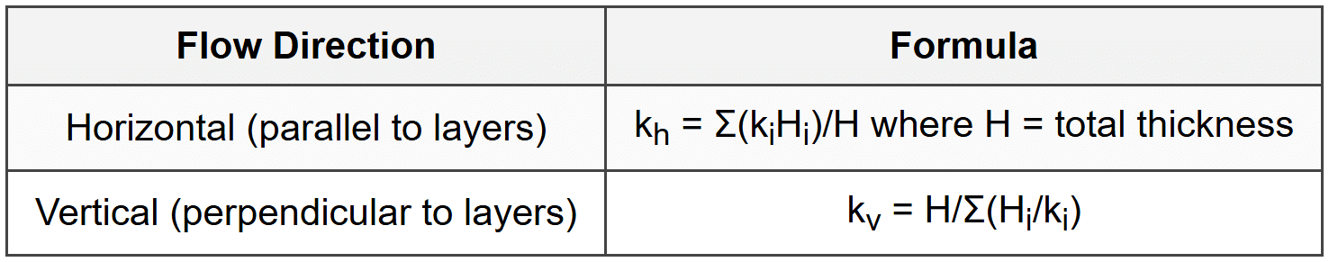
2.3 Layered Soil Hydraulic Conductivity

2.4 Flow Nets

• Flow lines and equipotential lines intersect at 90°
• Flow rate per unit width: q = kh(N_f/N_d) where N_f = number of flow channels, N_d = number of potential drops, h = total head loss
• Head loss between equipotentials: Δh = h/N_d
• Pressure head at any point: h_p = h - Δh × (number of drops to point) - elevation head
• Exit gradient: i_exit = h/(N_d × Δl) where Δl = length of last flow element at exit

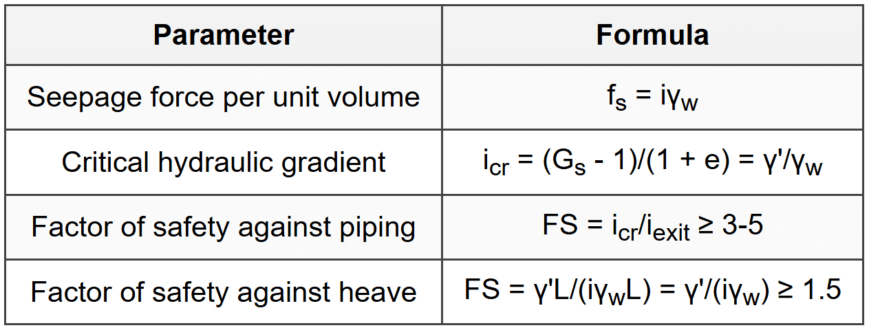
2.5 Seepage Force and Piping

3. Stresses in Soil

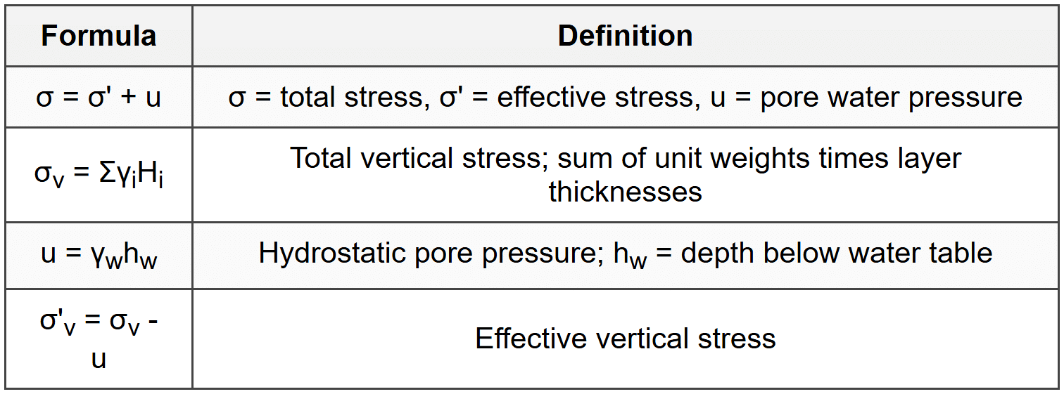
3.1 Effective Stress Principle

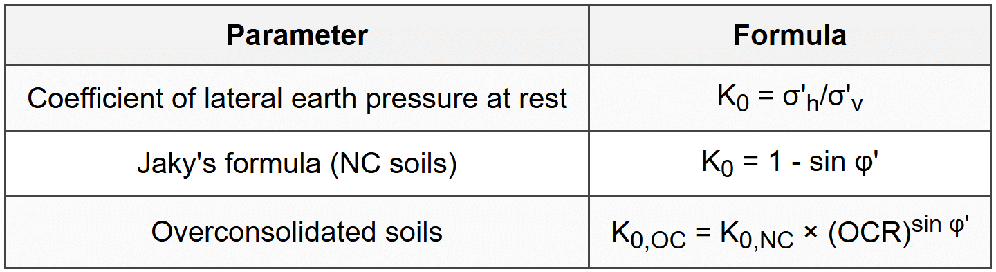
3.2 At-Rest Earth Pressure

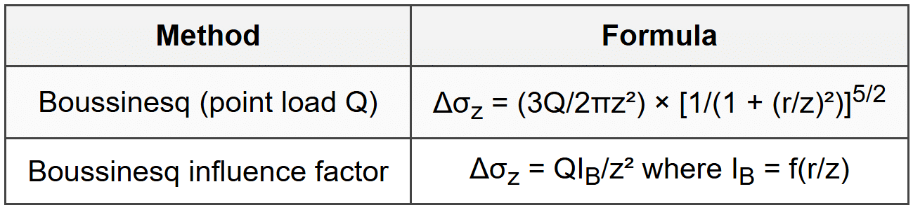
3.3 Vertical Stress Increase - Point Load

3.4 Vertical Stress Increase - Distributed Loads

3.4.1 Circular Area (radius R, uniform load q)

• Below center: Δσ_z = q[1 - 1/(1 + (R/z)²)^3/2]

3.4.2 Rectangular Area (Newmark Chart Method)

• Use influence value I for rectangular area with dimensions m = B/z and n = L/z
• Δσ_z = qI where I = f(m, n) from charts or equations
• For corner of rectangle: I = (1/4π)[2mn√(m²+n²+1)/(m²+n²+m²n²+1) × (m²+n²+1)/(m²+n²+1-m²n²) + tan⁻¹(2mn√(m²+n²+1)/(m²+n²+1-m²n²))]

3.4.3 2:1 Method (Approximate)

• Δσ_z = qBL/[(B + z)(L + z)] at depth z below uniformly loaded rectangular area B × L
• Assumes load spreads at 2V:1H slope

3.5 Westergaard Solution

• For stratified soils with alternating stiff and soft layers (k_h >> k_v)
• Δσ_z = Q/z² × 1/[π(1 + 2(r/z)²)^3/2] for point load
• Gives lower stress values than Boussinesq

4. Consolidation and Settlement

4.1 Compressibility Parameters

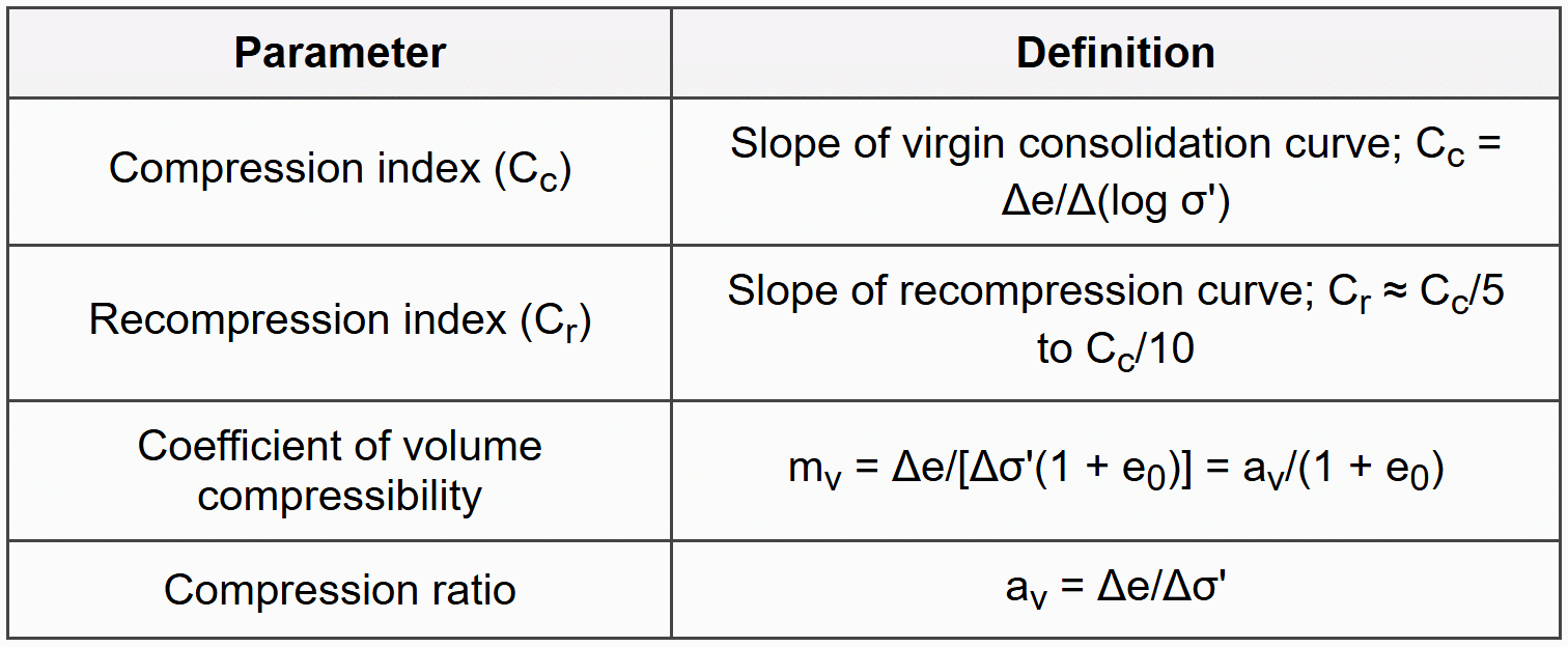
4.1.1 Empirical Correlations for C_c

• C_c ≈ 0.009(LL - 10) for remolded clays
• C_c ≈ 0.007(LL - 7) for undisturbed clays
• C_c ≈ 0.30(e₀ - 0.27) for NC clays

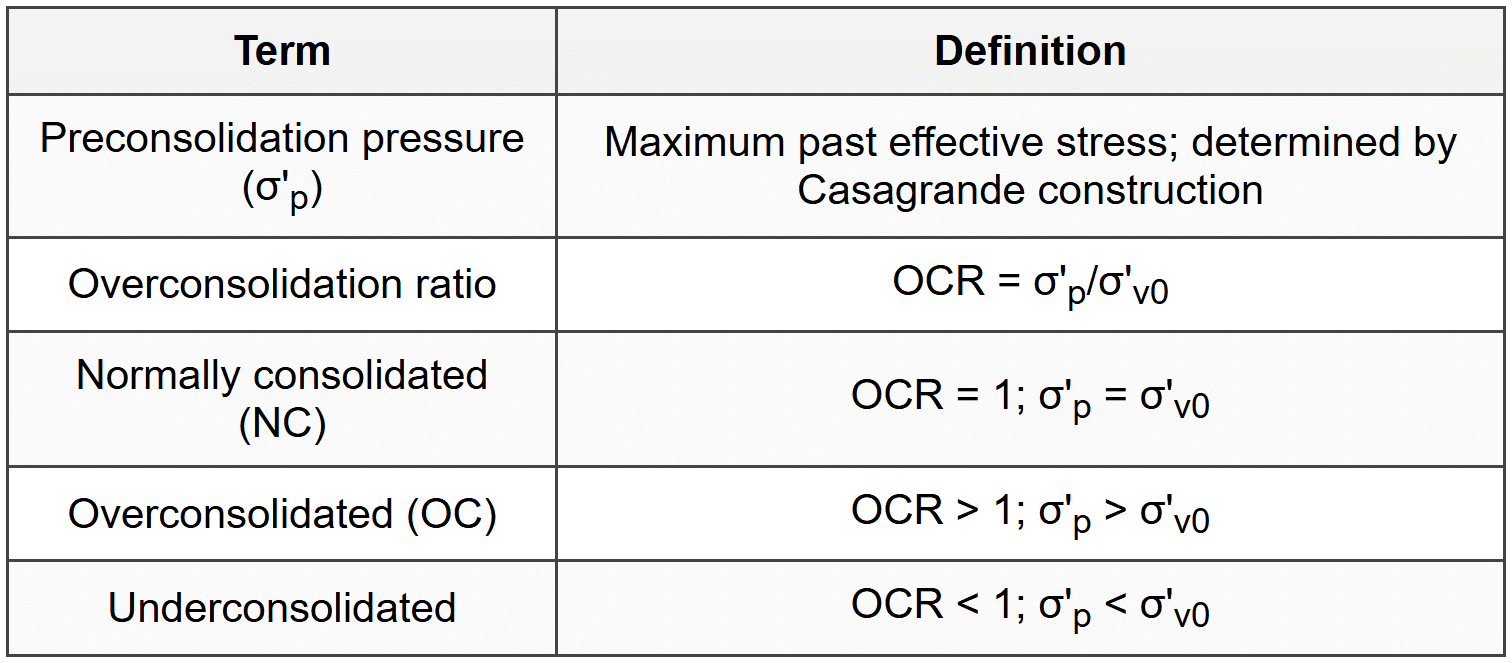
4.2 Preconsolidation Pressure

4.3 Settlement Calculation

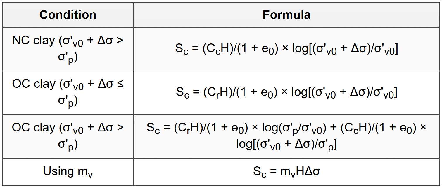
4.3.1 Primary Consolidation Settlement

4.3.2 Secondary Compression Settlement

• S_s = C_αH log(t/t_p) where C_α = secondary compression index, t_p = time at end of primary consolidation
• C_α ≈ 0.02C_c to 0.06C_c for inorganic clays
• C_α/C_c ≈ 0.04 ± 0.01 for inorganic clays and silts

4.3.3 Immediate (Elastic) Settlement

• S_e = qBI_sI_f(1 - μ²)/E_s
• I_s = shape factor; I_f = embedment factor; μ = Poisson's ratio; E_s = elastic modulus
• For flexible circular area: I_s = 1 at center, 0.64 at edge, 0.85 average
• For rigid circular area: I_s = 0.79 (uniform settlement)

4.4 Rate of Consolidation

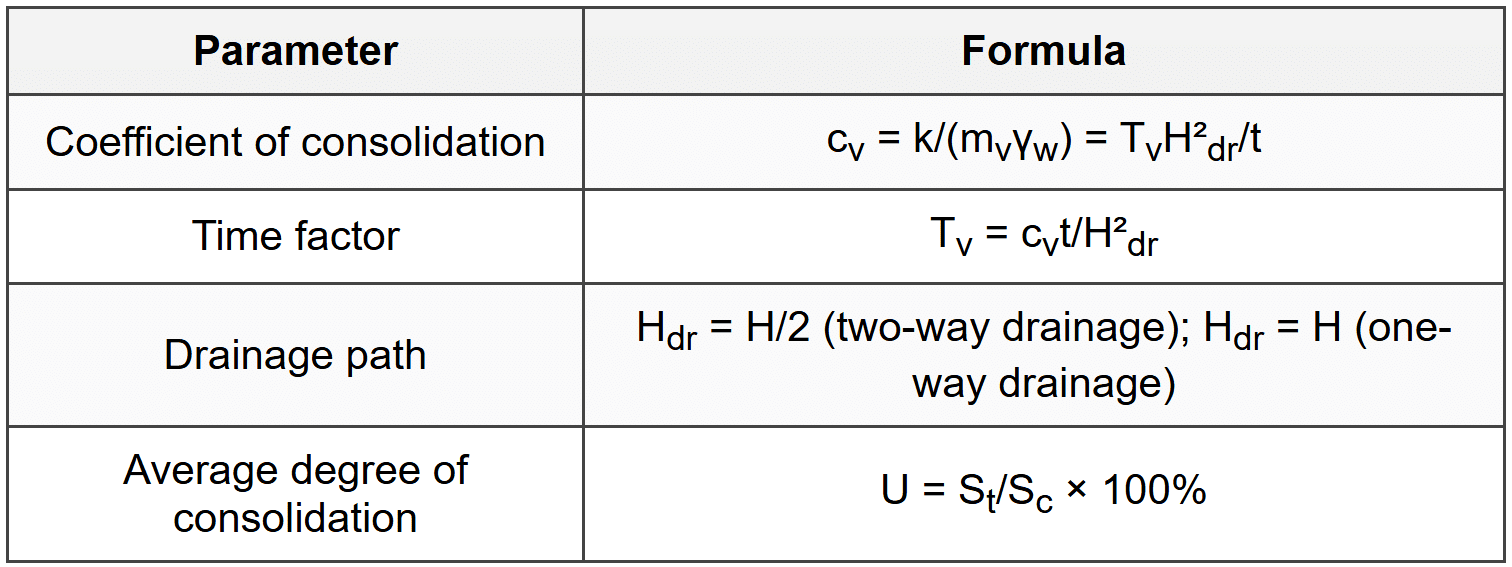
4.4.1 Time Factor Relationships

• U < 60%: T_v = (π/4)(U/100)²
• U > 60%: T_v = 1.781 - 0.933 log(100 - U)
• U = 50%: T_v = 0.197
• U = 90%: T_v = 0.848

4.4.2 Determining c_v from Lab Test

• Log-time method: c_v = 0.197H²_dr/t₅₀
• Square root time method: c_v = 0.848H²_dr/t₉₀

5. Shear Strength

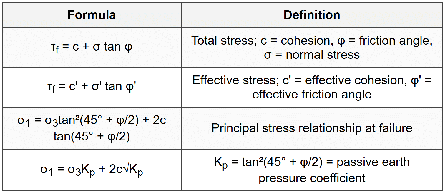
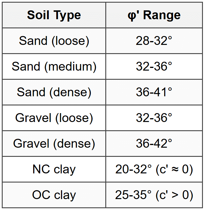
5.1 Mohr-Coulomb Failure Criterion

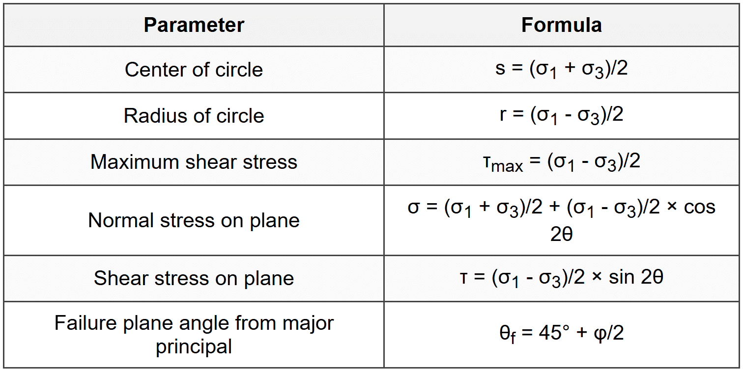
5.2 Mohr Circle Relationships

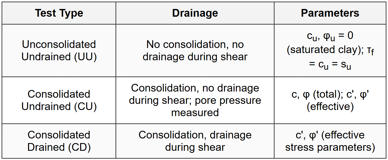
5.3 Laboratory Shear Tests

5.4 Undrained Shear Strength

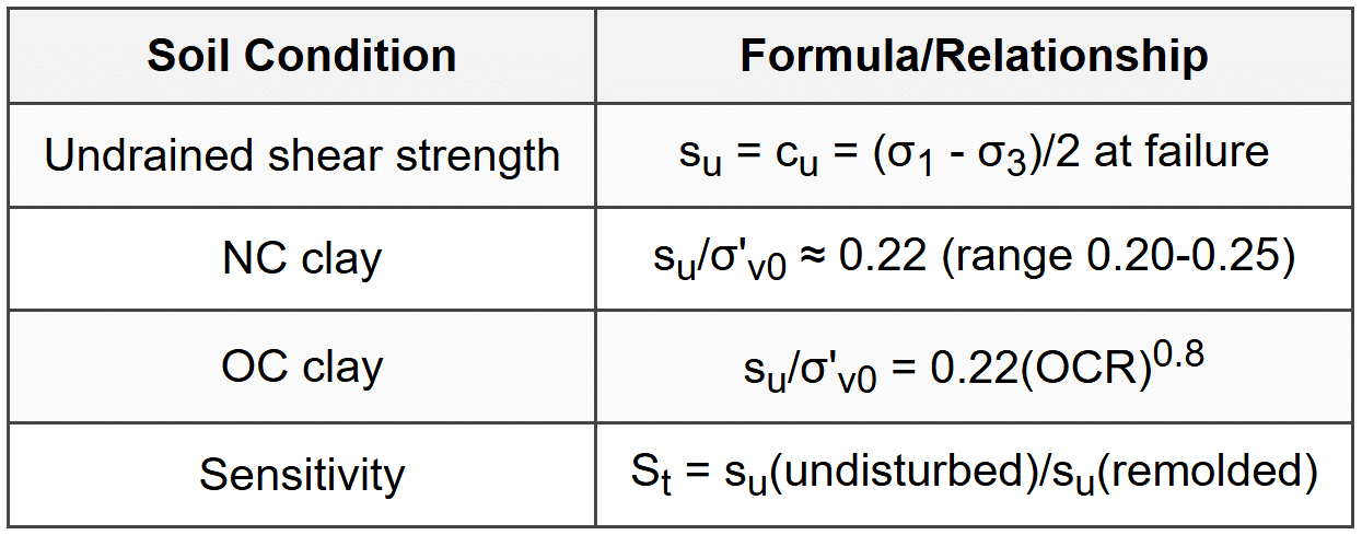
5.4.1 Sensitivity Classification

• S_t = 1: Insensitive; S_t = 2-4: Low sensitivity; S_t = 4-8: Medium; S_t = 8-16: Sensitive; S_t > 16: Extra sensitive (quick clay)

5.5 Drained Shear Strength

5.6 Correlations with SPT and CPT

5.6.1 SPT Correlations

• Granular soils: φ' ≈ 28° + 15(N₆₀)^0.5 - 15 (Schmertmann)
• φ' ≈ 27.1 + 0.3N₆₀ - 0.00054(N₆₀)² (Peck, Hanson, Thornburn)
• Clays: s_u (kPa) ≈ 6N₆₀ (rough estimate)

5.6.2 CPT Correlations

• Clays: s_u = (q_c - σ_v)/N_k where N_k ≈ 10-20
• Sands: friction angle from charts using normalized cone resistance Q_tn

5.7 Stress Path

• p = (σ₁ + σ₃)/2; q = (σ₁ - σ₃)/2
• p' = (σ'₁ + σ'₃)/2; q = (σ'₁ - σ'₃)/2
• Total stress path (TSP): plot of (p, q) points
• Effective stress path (ESP): plot of (p', q) points
• Failure envelope in p-q space: q = p tan α + d where α = sin⁻¹(sin φ/(1 + sin φ))

6. Lateral Earth Pressure

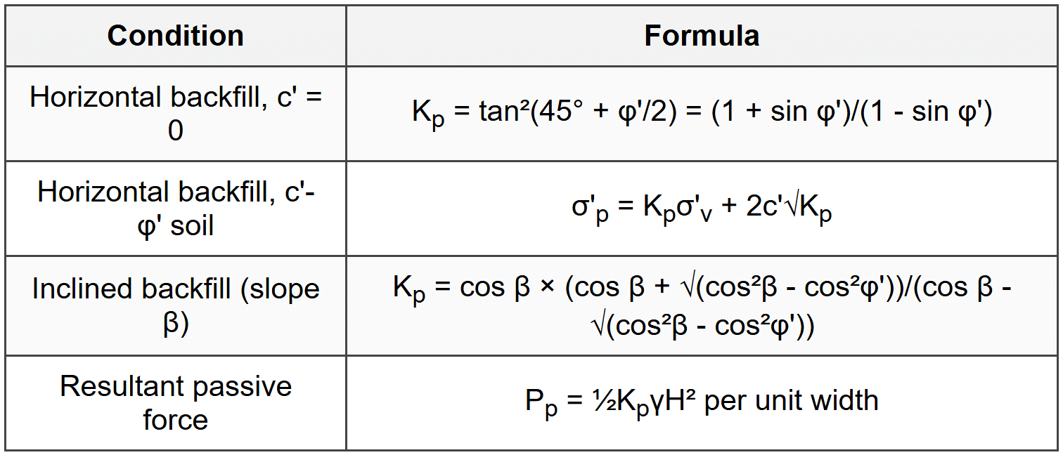
6.1 Rankine Theory

6.1.1 Active Pressure

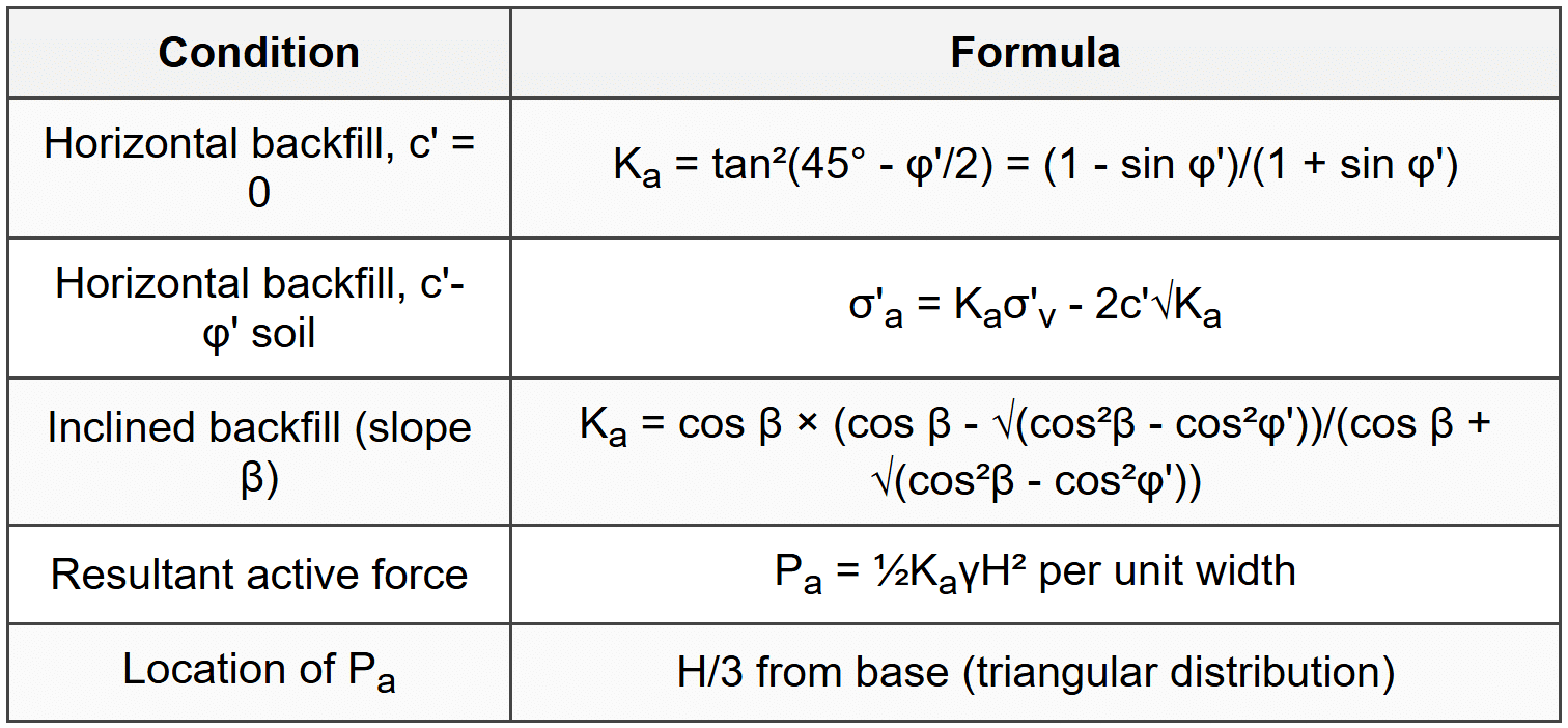
6.1.2 Passive Pressure

6.2 Coulomb Theory

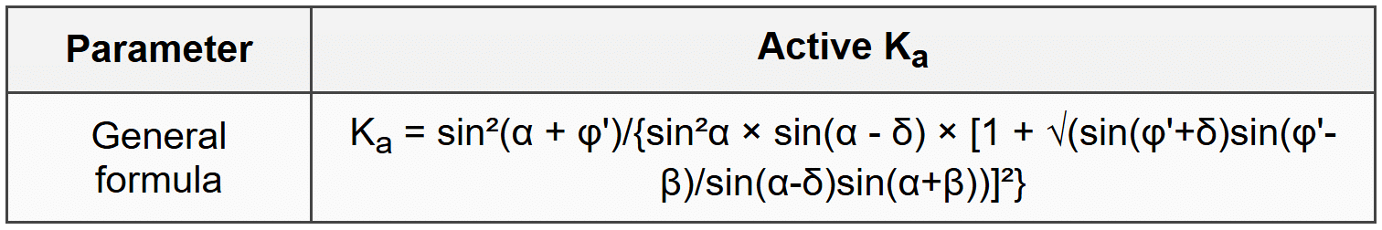
• α = wall angle from horizontal; β = backfill slope; δ = wall friction angle; φ' = soil friction
• For vertical wall (α = 90°), horizontal backfill (β = 0), δ = 0: reduces to Rankine
• Wall friction: δ ≈ 0.5φ' to 0.67φ' for concrete on gravel; δ ≈ 0.67φ' to φ' for rough surfaces
• Passive K_p: similar equation with reversed signs in square root term

6.3 Earth Pressure with Surcharge

• Uniform surcharge q: Δσ_h = Kq (adds constant horizontal pressure)
• Point load: use Boussinesq or charts for lateral stress distribution
• Line load: σ_h = 2qK/π × [x²/(x² + z²)] where x = horizontal distance, z = depth

6.4 Water Pressure Effects

• Total lateral pressure = effective earth pressure + pore water pressure
• σ_h = K_a(γ_sat - γ_w)z + γ_wz = K_aγ'z + γ_wz
• For drained backfill: use effective unit weight and add separate water pressure
• For undrained clay: use total stress analysis with φ_u = 0

7. Slope Stability

7.1 Infinite Slope Analysis

7.1.1 Dry or Moist Soil

• FS = tan φ'/tan β where β = slope angle
• FS = c'/(γz sin β cos β) + tan φ'/tan β for c'-φ' soil

7.1.2 Seepage Parallel to Slope

• FS = γ' tan φ'/(γ_sat tan β) = (γ_sat - γ_w) tan φ'/(γ_sat tan β)

7.1.3 Submersion

• FS = γ' tan φ'/[(γ_sat - γ_w) tan β] (cancel to tan φ'/tan β)

7.2 Ordinary Method of Slices (Fellenius)

• FS = Σ[c'L + (W cos α - uL) tan φ']/Σ(W sin α)
• W = weight of slice; α = base angle; L = arc length of slice base; u = pore pressure
• Assumes interslice forces are parallel to slice base (neglects interslice shear)
• Conservative method; underestimates FS by 5-20%

7.3 Simplified Bishop Method

• FS = Σ{[c'b + (W - ub) tan φ']/m_α}/Σ(W sin α)
• m_α = cos α + (sin α tan φ')/FS (iterative solution required)
• b = slice width; assumes interslice shear forces are zero
• Accurate for circular failures; within 1% of rigorous methods

7.4 φ_u = 0 Analysis (Undrained Clay)

• FS = Σ(c_uL)/Σ(W sin α) for ordinary method
• For homogeneous slope: FS = c_uN_s/(γH) where N_s = stability number from charts
• N_s = f(slope angle, depth factor) from Taylor charts
• Critical circle typically passes through toe for slope ≥ 53°

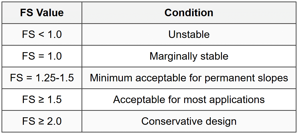
7.5 Factor of Safety Interpretation

7.6 Seismic Slope Stability (Pseudostatic)

• Add horizontal force k_hW and vertical force k_vW to each slice
• k_h = horizontal seismic coefficient (0.1-0.5 for various seismic zones)
• k_v = vertical seismic coefficient (often 0 or k_h/2)
• Modified FS equation: add ±k_hW and ±k_vW terms to force summation

8. Site Characterization

8.1 Standard Penetration Test (SPT)

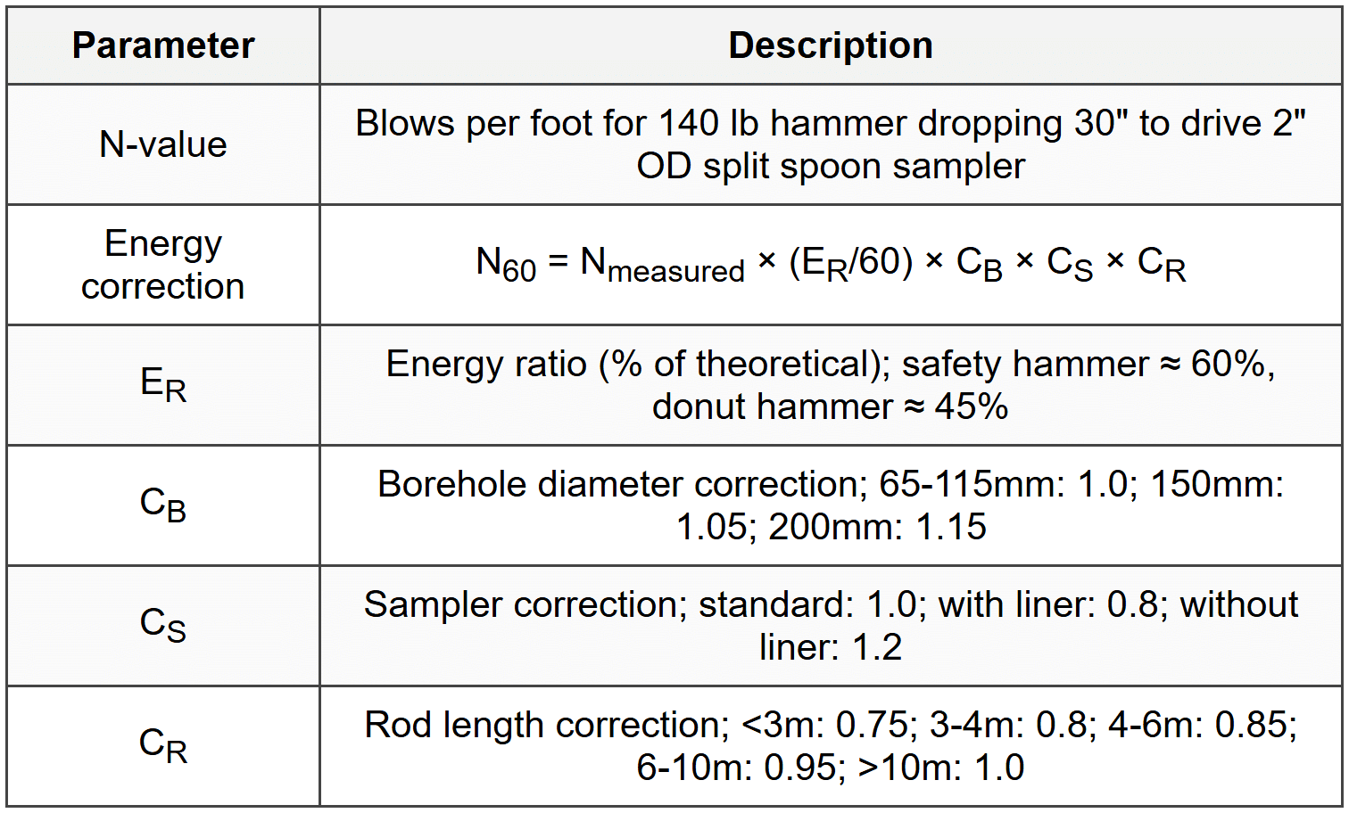
8.1.1 Overburden Correction for Sands

• (N₁)₆₀ = N₆₀ × C_N where C_N = overburden correction factor
• C_N = (P_a/σ'_v)^0.5 (Liao and Whitman); P_a = 100 kPa or 1 tsf
• C_N ≤ 2.0 (cap correction factor)
• Alternative: C_N = 0.77 log(1920/σ'_v) where σ'_v in kPa

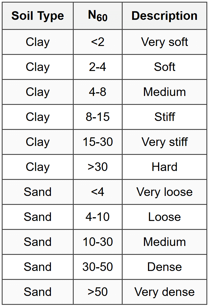
8.1.2 SPT Consistency/Density Correlations

8.2 Cone Penetration Test (CPT)

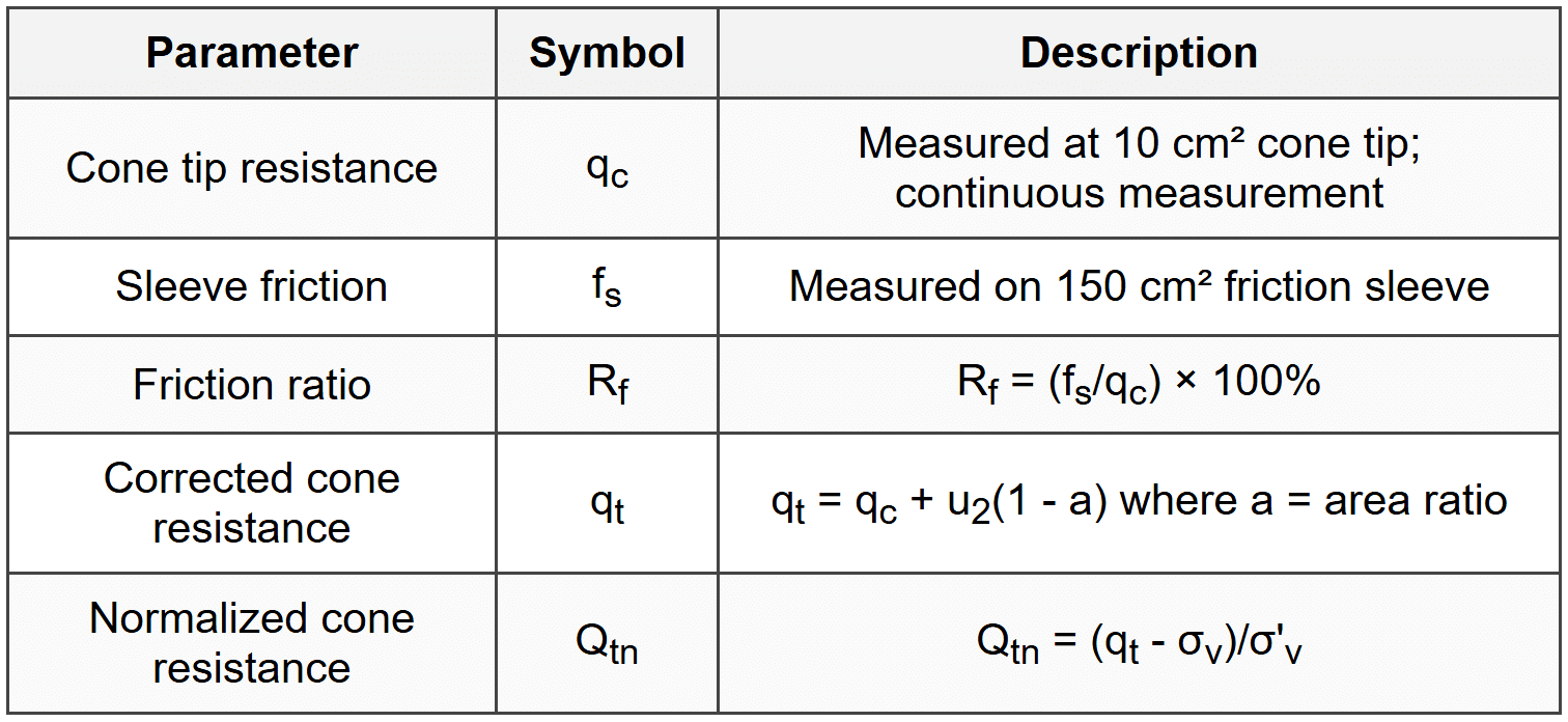
8.2.1 Soil Behavior Type from CPT

• R_f < 1%: Gravelly sand to sand
• R_f = 1-2%: Sands, silty sand to sandy silt
• R_f = 2-4%: Clayey silt to silty clay
• R_f > 4%: Silty clay to clay
• Use Robertson soil behavior type charts (Q_tn vs F_r) for detailed classification

8.3 Vane Shear Test

• In-situ measurement of undrained shear strength in soft to medium clays
• s_u = T/(πD²H/2 + πD³/6) where T = applied torque, D = vane diameter, H = vane height
• For H = 2D: s_u = T/(3.66D³)
• Correction for strain rate and anisotropy: s_u(corrected) = μ × s_u(field) where μ = 0.7-1.0
• Bjerrum correction: μ ≈ 1.7 - 0.54 log(PI) for PI > 5

8.4 Pressuremeter Test (PMT)

• Measures in-situ stress-strain behavior by expanding cylindrical probe
• Pressuremeter modulus: E_p = 2(1 + μ)(V₀ + V_m)Δp/ΔV
• Limit pressure p_L: pressure at cavity expansion equal to initial volume
• Useful for settlement analysis: E_s ≈ E_p/α where α = rheological coefficient (2-3)

8.5 Dilatometer Test (DMT)

• Flat blade with expandable membrane; measures p₀ (lift-off) and p₁ (1.1 mm expansion)
• Material index: I_D = (p₁ - p₀)/(p₀ - u₀)
• Horizontal stress index: K_D = (p₀ - u₀)/σ'_v0
• Dilatometer modulus: E_D = 34.7(p₁ - p₀)
• Soil classification: I_D < 0.6 clay; 0.6-1.8 silt; 1.8-3.3 sand; >3.3 gravel

9. Bearing Capacity

9.1 Terzaghi Bearing Capacity

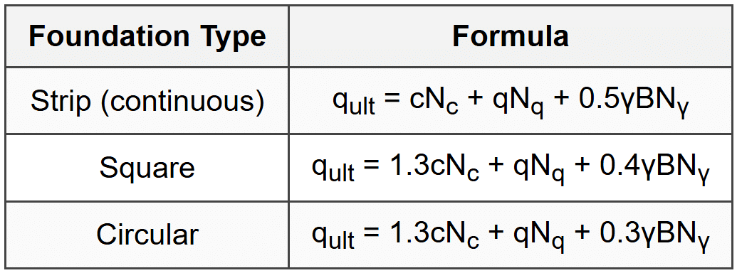
• q = effective overburden pressure at base level = γD_f
• B = width (least dimension); c = cohesion; γ = unit weight of soil below base
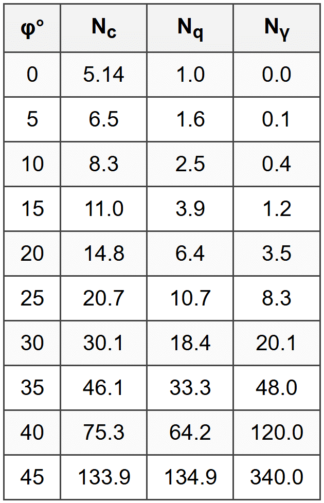
• N_c, N_q, N_γ = bearing capacity factors (functions of φ)
• For local shear failure: use c' = 2c/3, φ' = tan⁻¹(2 tan φ/3), then apply factors to N'_c, N'_q, N'_γ

9.2 Meyerhof Bearing Capacity Factors

9.3 General Bearing Capacity Equation

• q_ult = cN_cF_csF_cdF_ci + qN_qF_qsF_qdF_qi + 0.5γBN_γF_γsF_γdF_γi
• F_cs, F_qs, F_γs = shape factors
• F_cd, F_qd, F_γd = depth factors
• F_ci, F_qi, F_γi = inclination factors

9.3.1 Shape Factors (Vesic/Meyerhof)

• F_cs = 1 + (B/L)(N_q/N_c)
• F_qs = 1 + (B/L) tan φ
• F_γs = 1 - 0.4(B/L)
• For square: B = L, so F_cs = 1 + N_q/N_c, F_qs = 1 + tan φ, F_γs = 0.6
• For circular: use equivalent square (B = L)

9.3.2 Depth Factors (Hansen)

• F_cd = 1 + 0.4(D_f/B) for D_f/B ≤ 1
• F_qd = 1 + 2 tan φ(1 - sin φ)²(D_f/B) for D_f/B ≤ 1
• F_γd = 1.0

9.4 Bearing Capacity for Shallow Foundations on Clay

• Undrained condition (φ_u = 0): q_ult = c_uN_cF_csF_cd + q
• For strip: q_ult = 5.14c_u + q
• For square/circular: q_ult = 6.17c_u + q (using F_cs ≈ 1.2)
• Skempton's formula for D_f/B ≤ 2.5: q_ult = c_uN_c + q where N_c = 5(1 + 0.2D_f/B)(1 + 0.2B/L)

9.5 Allowable Bearing Capacity

• q_all = q_ult/FS where FS = 2.5-3.0 for normal conditions
• q_net,ult = q_ult - q (net ultimate bearing capacity)
• q_net,all = q_net,ult/FS
• Check both bearing capacity failure and settlement criteria

9.6 Bearing Capacity from SPT and CPT

9.6.1 SPT Correlations

• Meyerhof (cohesionless): q_all (kPa) = 12N₆₀(B + 0.3)²/B² × (D_f/B + 0.33) for 25 mm settlement
• Terzaghi-Peck: q_all (ksf) = N/4 for B ≤ 4 ft

9.6.2 CPT Correlations

• Schmertmann: q_all = (q_c - σ_v)/F_d where F_d = depth factor ≈ 2.5
• Direct method: q_ult ≈ q_c/20 to q_c/30 for shallow foundations

10. Deep Foundations

10.1 Single Pile Capacity

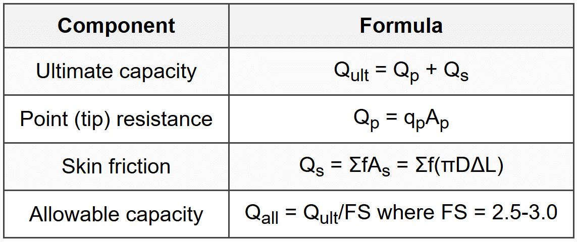
10.2 Pile Capacity in Sand (Effective Stress Method)

10.2.1 Point Resistance

• q_p = σ'_vN_q where σ'_v = effective stress at pile tip
• N_q from charts (Berezantsev, Meyerhof, Vesic); N_q ≈ 12-80 for φ = 30-40°
• Limit q_p to 50N_q (in bar) to 100N_q for dense sand
• For driven piles: q_p ≤ 200-400 bar (20-40 MPa)

10.2.2 Skin Friction

• f = βσ'_v (β-method) where β = K tan δ
• K = coefficient of lateral earth pressure ≈ K₀ to 2K₀ for driven piles; 0.7K₀ for drilled shafts
• δ = pile-soil friction angle ≈ 0.5φ to φ (steel); 0.7φ to φ (concrete); φ (timber)
• β ≈ 0.15-0.35 for loose sand; 0.25-0.50 for dense sand
• Alternative: f = Kσ'_v tan φ where K decreases with depth

10.3 Pile Capacity in Clay (Total Stress Method)

10.3.1 Point Resistance

• q_p = c_uN_c where N_c = 9 (deep foundation)
• Use c_u at pile tip depth

10.3.2 Skin Friction (α-Method)

• f = αc_u where α = adhesion factor (0 to 1)
• α ≈ 1.0 for c_u < 25 kPa
• α ≈ 0.5 for c_u = 50-100 kPa
• α ≈ 0.3-0.4 for c_u > 100 kPa
• Tomlinson: α = 0.45 for driven piles in NC clay
• For c_u > 70 kPa: α = 0.9/(c_u/P_a)^0.5 where P_a = 100 kPa

10.4 λ-Method (Effective Stress for Clay)

• f = λ(σ'_v + 2c_u)
• λ = 0.15-0.35 depending on OCR and depth
• Accounts for both effective stress and cohesion

10.5 Pile Capacity from SPT

10.5.1 Meyerhof Method

• Cohesionless: q_p (kPa) = 40N₆₀L/D ≤ 400N₆₀ where L = embedded length, D = diameter
• f (kPa) = 2N₆₀ (limit to 100 kPa)
• Cohesive: q_p (kPa) = 40N₆₀ (limit to 400N₆₀); f (kPa) = N₆₀

10.6 Pile Capacity from CPT

• Direct method: q_p = q_c (average q_c near pile tip)
• f = q_c/F_s where F_s = 50-200 (sand); 50-150 (clay)
• Schmertmann: average q_c over 8D below to 3D above pile tip for q_p
• LCPC method: uses detailed charts with soil type classification

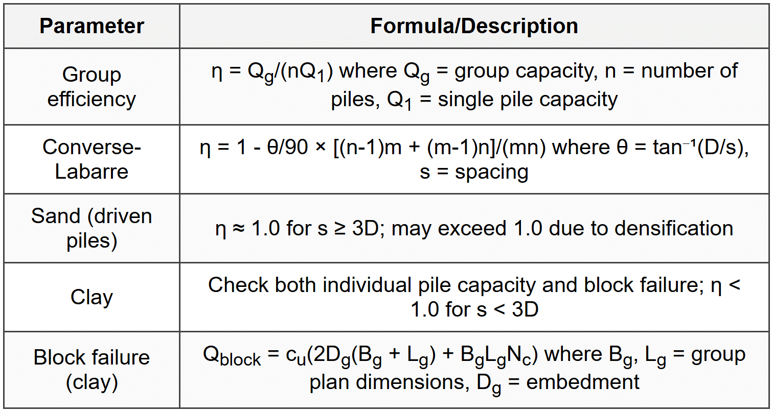
10.7 Pile Group Capacity

10.8 Negative Skin Friction (Downdrag)

• Occurs when soil settles relative to pile (consolidating fill, lowered water table)
• Q_n = Σf_nA_s over downdrag zone
• f_n = Kσ'_v tan δ (sand); f_n = αc_u (clay)
• Design load = Q_applied + Q_n (downdrag adds to load)
• Neutral plane at depth where pile and soil movement are equal

10.9 Pile Settlement

• Elastic compression: s = (Q_pL)/(A_pE_p) + (Q_sL)/(2A_pE_p) + (Q_pD)/(A_pE_sq_p)
• First term = compression of pile shaft under tip load; second term = compression under skin friction; third term = soil compression below tip
• E_p = pile elastic modulus; E_s = soil modulus; D = pile width
• For group: settlement > single pile; analyze as equivalent raft foundation

10.10 Lateral Pile Capacity

• Broms method for short rigid piles (L/D < 10 typically)
• P-y curve method for flexible piles (computer analysis required)
• Ultimate lateral resistance (clay): p_u = 9c_uD (deep); p_u = 3c_uD(1 + γ'z/c_u) (shallow)
• Ultimate lateral resistance (sand): p_u = 3K_pγ'z D (deep)