Cheatsheet: Feedback Systems

1. Feedback System Fundamentals

1.1 Basic Definitions

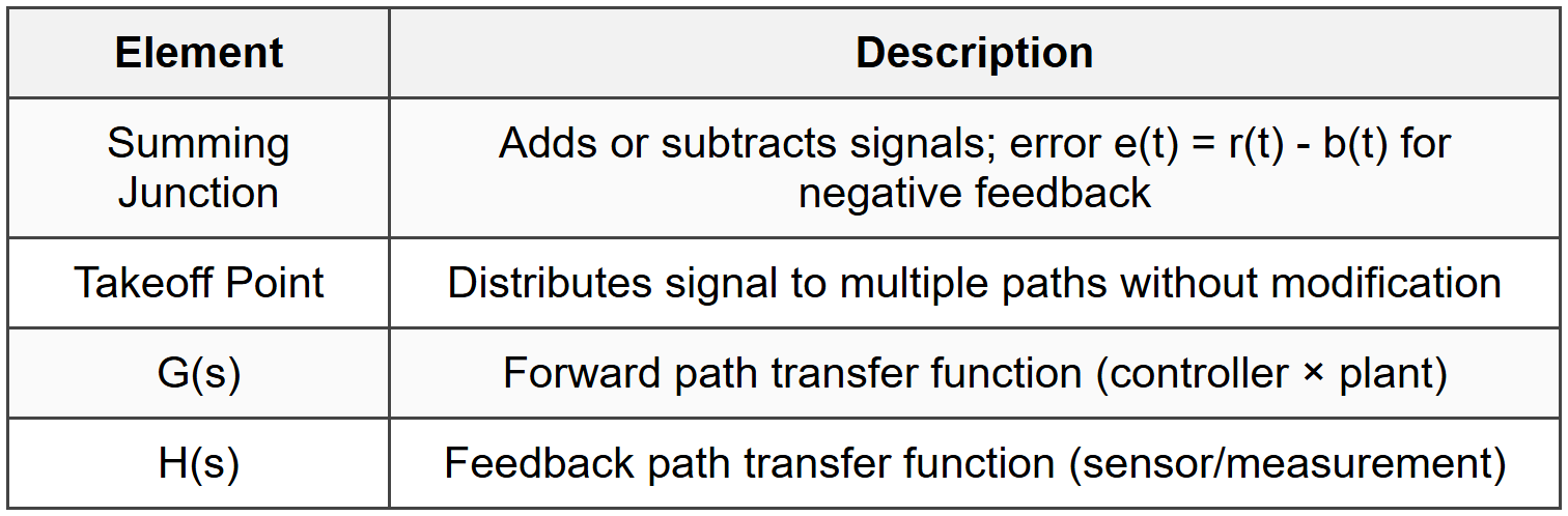
1.2 Block Diagram Components

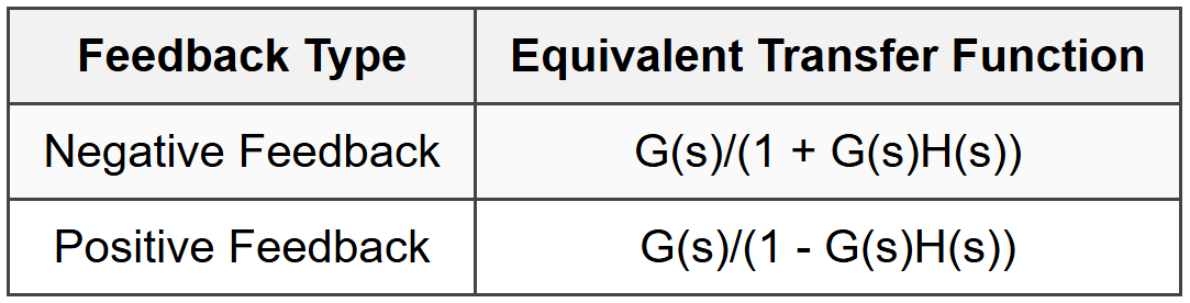
1.3 Standard Feedback Configuration

• Closed-loop transfer function: T(s) = C(s)/R(s) = G(s)/(1 + G(s)H(s))
• Error transfer function: E(s)/R(s) = 1/(1 + G(s)H(s))
• Open-loop transfer function: L(s) = G(s)H(s)
• Characteristic equation: 1 + G(s)H(s) = 0
• For unity feedback (H(s) = 1): T(s) = G(s)/(1 + G(s))

2. Block Diagram Algebra

2.1 Series Connection

• Equivalent transfer function: G(s) = G₁(s) × G₂(s) × ... × Gₙ(s)
• Output of first block becomes input to second block

2.2 Parallel Connection

• Equivalent transfer function: G(s) = G₁(s) ± G₂(s) ± ... ± Gₙ(s)
• Same input applied to all blocks; outputs summed algebraically

2.3 Feedback Loop Reduction

2.4 Moving Summing Junctions and Takeoff Points

• Moving summing junction past block G(s): add 1/G(s) or G(s) to maintain equivalence
• Moving takeoff point past block G(s): add G(s) or 1/G(s) in branch to maintain equivalence
• Summing junctions in series can be combined by algebraic addition
• Adjacent takeoff points can be interchanged without affecting system

3. Signal Flow Graphs

3.1 Signal Flow Graph Elements

3.2 Mason's Gain Formula

• Transfer function: T = (1/Δ) × Σ(Pₖ × Δₖ), summed over all k forward paths
• Δ = 1 - Σ(individual loops) + Σ(2 non-touching loops) - Σ(3 non-touching loops) + ...
• Pₖ = path gain of kth forward path (product of all branch gains in path)
• Δₖ = cofactor of Δ for kth path (Δ with loops touching kth path removed)
• Non-touching loops: loops that share no common nodes

3.3 Mason's Formula Application Steps

1. Identify all forward paths and calculate path gains Pₖ
2. Identify all individual loops and calculate loop gains
3. Identify all combinations of 2, 3,... non-touching loops
4. Calculate Δ using loop gains
5. For each forward path, determine Δₖ by removing loops touching that path
6. Apply Mason's formula: T = (1/Δ) × Σ(Pₖ × Δₖ)

4. System Types and Steady-State Error

4.1 System Type Classification

• System type N = number of pure integrators (poles at s = 0) in open-loop transfer function G(s)H(s)
• Type 0: No poles at origin (N = 0)
• Type 1: One pole at origin (N = 1)
• Type 2: Two poles at origin (N = 2)
• Higher type number indicates better steady-state accuracy

4.2 Static Error Constants

4.3 Steady-State Error Formulas

4.3.1 For Unity Feedback (H(s) = 1)

• e_ss = lim(s→0) s × E(s) where E(s) = R(s)/(1 + G(s))
• Step input (r(t) = A): e_ss = A/(1 + Kₚ)
• Ramp input (r(t) = At): e_ss = A/Kᵥ
• Parabolic input (r(t) = At²/2): e_ss = A/Kₐ

4.4 Steady-State Error by System Type

5. Stability Analysis

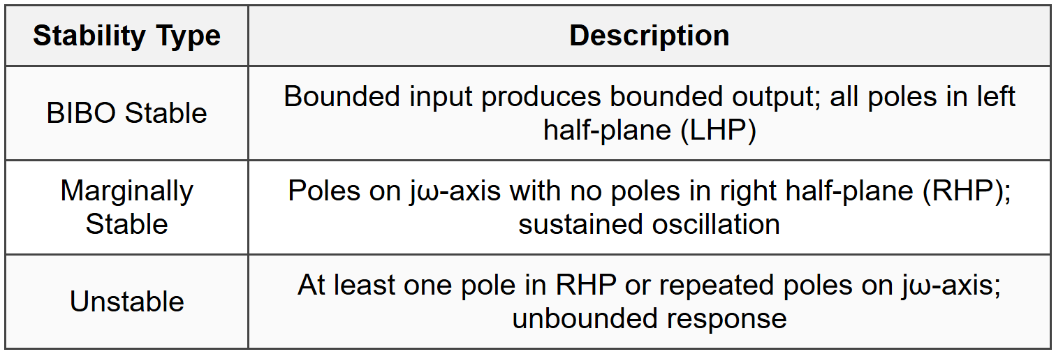
5.1 Stability Definitions

5.2 Routh-Hurwitz Stability Criterion

5.2.1 Standard Routh Array Construction

• Characteristic equation: aₙsⁿ + aₙ₋₁sⁿ⁻¹ + ... + a₁s + a₀ = 0
• First row: aₙ, aₙ₋₂, aₙ₋₄, ...
• Second row: aₙ₋₁, aₙ₋₃, aₙ₋₅, ...
• Subsequent rows: b₁ = (aₙ₋₁×aₙ₋₂ - aₙ×aₙ₋₃)/aₙ₋₁
• Number of RHP poles = number of sign changes in first column
• System stable if all elements in first column are positive (no sign changes)

5.2.2 Special Cases

• Zero in first column (other elements non-zero): replace zero with small ε > 0, complete array, take limit as ε → 0⁺
• Entire row of zeros: indicates symmetric roots; form auxiliary equation from previous row, differentiate, use coefficients for next row
• Auxiliary equation roots are also roots of characteristic equation

5.3 Relative Stability

• Gain margin (GM): factor by which gain can increase before instability
• Phase margin (PM): additional phase lag at gain crossover before instability
• Damping ratio ζ relates to phase margin: PM ≈ 100ζ degrees (for 0.4 < ζ=""><>

6. Root Locus Analysis

6.1 Root Locus Fundamentals

• Root locus: plot of closed-loop poles as gain K varies from 0 to ∞
• Characteristic equation: 1 + KG(s)H(s) = 0 or KG(s)H(s) = -1
• Angle condition: ∠G(s)H(s) = ±180°(2k + 1), k = 0, 1, 2, ...
• Magnitude condition: |KG(s)H(s)| = 1
• Number of branches = number of poles of G(s)H(s)

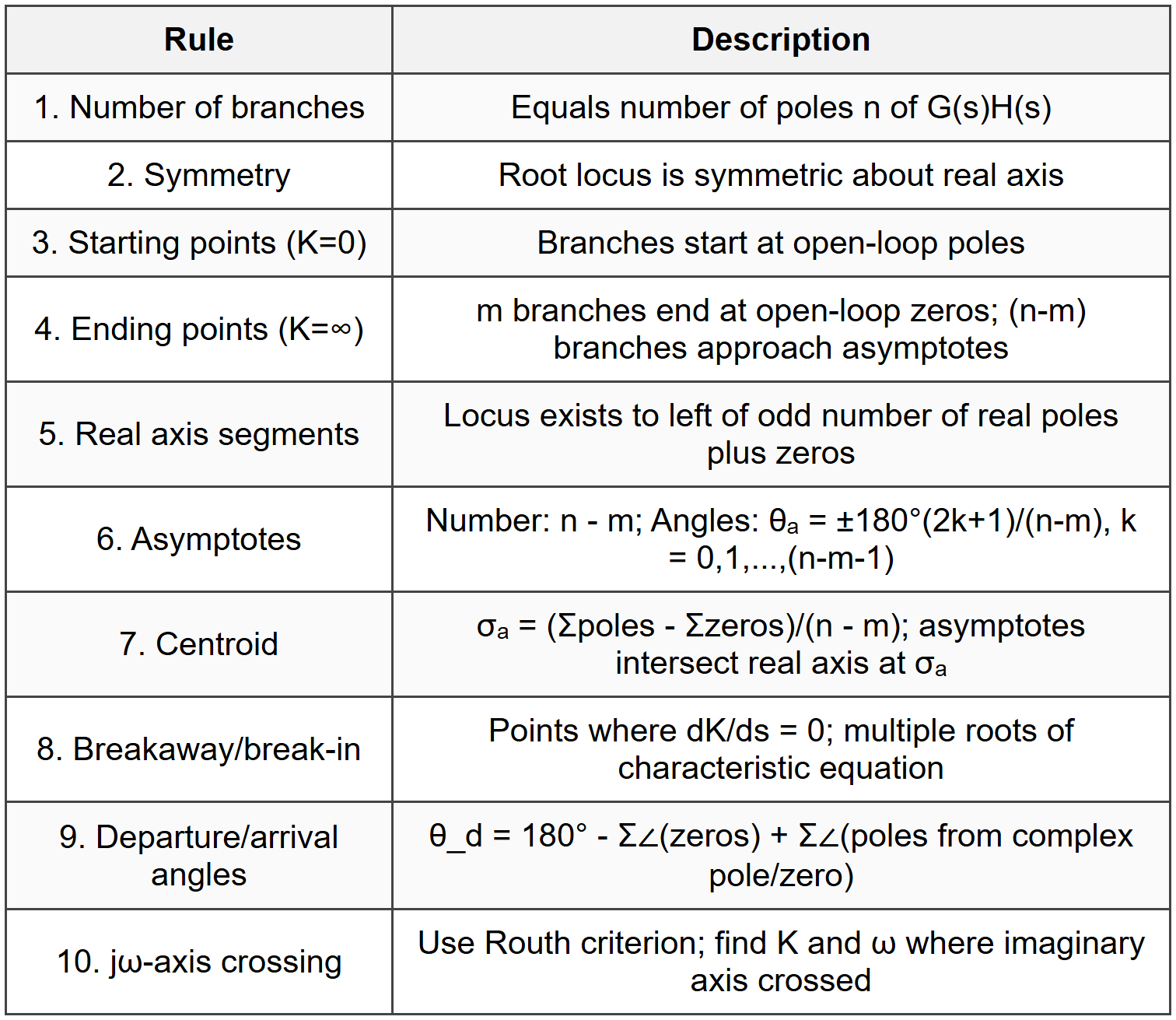
6.2 Root Locus Construction Rules

6.3 Key Root Locus Calculations

• Gain at any point s₁: K = 1/|G(s₁)H(s₁)| = ∏|s₁ - poles|/∏|s₁ - zeros|
• Breakaway points on real axis: solve dK/ds = 0 or d[G(s)H(s)]/ds = 0
• Damping ratio from root location: ζ = cos(θ) where θ = angle from positive real axis

7. Frequency Response Analysis

7.1 Frequency Response Basics

• Frequency response: steady-state output of stable system to sinusoidal input
• Input: r(t) = A sin(ωt); Output: c(t) = A|G(jω)| sin(ωt + ∠G(jω))
• Magnitude ratio: M(ω) = |G(jω)| = |C(jω)|/|R(jω)|
• Phase angle: φ(ω) = ∠G(jω)
• Decibel: M_dB = 20 log₁₀|G(jω)|

7.2 Bode Plot Construction

7.2.1 Standard Transfer Function Form

• G(jω) = K(1+jωT₁)(1+jωT₂)... / [(jω)ᴺ(1+jωTₐ)(1+jωTᵦ)...]
• Plot magnitude (dB) and phase (degrees) vs. log frequency

7.2.2 Basic Factor Contributions

7.2.3 Second-Order Factor Details

• Resonant peak: M_r = 1/(2ζ√(1-ζ²)) for ζ <>
• Resonant frequency: ω_r = ωₙ√(1-2ζ²) for ζ <>
• Corner frequency = ωₙ

7.3 Gain and Phase Margins from Bode Plot

• Stable system: GM > 1 (GM_dB > 0) and PM > 0°
• Typical specs: GM > 6 dB, PM > 30° to 60°

7.4 Nyquist Plot

7.4.1 Nyquist Plot Basics

• Polar plot of G(jω)H(jω) for -∞ < ω=""><>
• Real part = Re[G(jω)H(jω)]; Imaginary part = Im[G(jω)H(jω)]
• Magnitude = |G(jω)H(jω)|; Angle = ∠G(jω)H(jω)

7.4.2 Nyquist Stability Criterion

• Nyquist contour: encloses entire RHP in s-plane
• Z = N + P where Z = closed-loop RHP poles, P = open-loop RHP poles, N = net encirclements of -1 point
• For stability: Z = 0, so N = -P
• If P = 0 (open-loop stable): no encirclements of -1 point for closed-loop stability
• Clockwise encirclement counted as positive N

7.4.3 Gain and Phase Margins from Nyquist

• GM: reciprocal of magnitude where plot crosses negative real axis
• PM: angle from negative real axis to point where |G(jω)H(jω)| = 1

8. Time Domain Specifications

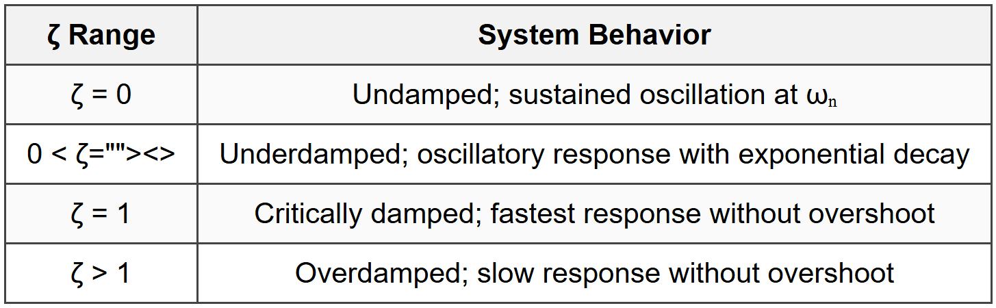
8.1 Standard Second-Order System

• Transfer function: T(s) = ωₙ²/(s² + 2ζωₙs + ωₙ²)
• ωₙ = undamped natural frequency (rad/s)
• ζ = damping ratio (dimensionless)
• Poles: s = -ζωₙ ± jωₙ√(1-ζ²)

8.2 Step Response Performance Specifications

8.3 Damping Ratio Effects

8.4 Dominant Pole Approximation

• Poles at least 5 times closer to jω-axis than other poles dominate response
• Higher-order system approximated by second-order dominant poles
• Valid when distant poles and zeros cancel or are far into LHP

9. Compensator Design

9.1 Compensator Types

9.2 PID Controller Effects

9.3 Lead Compensator Design

• Purpose: improve transient response and increase phase margin
• Maximum phase lead: φ_max = sin⁻¹((1-α)/(1+α)) at ω_m = 1/(T√α)
• Place ω_m at new gain crossover frequency
• Lead adds positive phase (phase lead) between 1/T and 1/(αT)
• Magnitude increases with frequency; select K to achieve 0 dB at ω_m

9.4 Lag Compensator Design

• Purpose: improve steady-state error without affecting transient response
• Increases low-frequency gain by factor β
• Corner frequencies 1/T and 1/(βT) placed well below gain crossover
• Phase lag effect minimized at gain crossover
• Select β to achieve desired error constant improvement

9.5 Compensator Selection Guide

• Use lead if transient response inadequate (low PM, high overshoot)
• Use lag if steady-state error too large but transient acceptable
• Use lead-lag if both transient and steady-state need improvement
• Use PID for general-purpose control with tunable parameters

10. State-Space Representation

10.1 State-Space Equations

• State equation: ẋ(t) = Ax(t) + Bu(t)
• Output equation: y(t) = Cx(t) + Du(t)
• x(t) = state vector (n×1); u(t) = input vector (r×1); y(t) = output vector (m×1)
• A = system matrix (n×n); B = input matrix (n×r); C = output matrix (m×n); D = feedthrough matrix (m×r)

10.2 Transfer Function from State-Space

• T(s) = C(sI - A)⁻¹B + D
• Characteristic equation: det(sI - A) = 0
• Eigenvalues of A are poles of transfer function

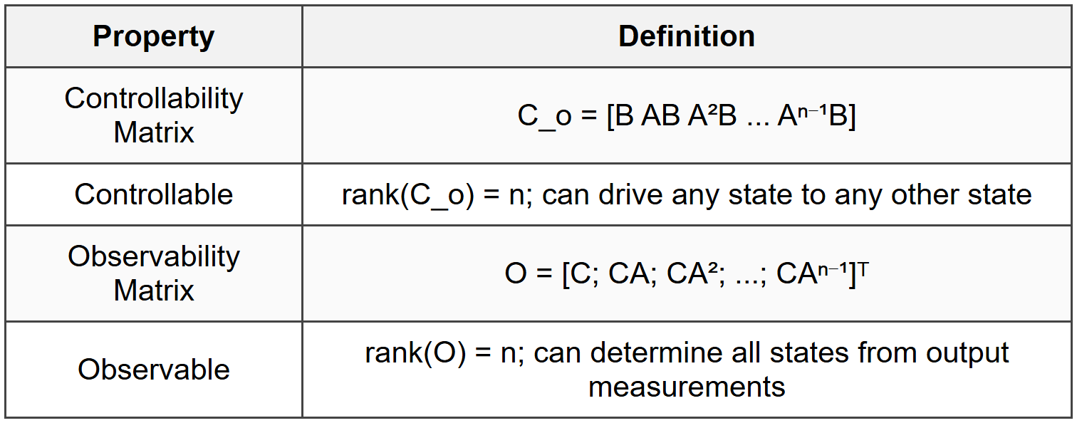
10.3 Controllability and Observability

10.4 State Feedback Control

• Control law: u(t) = -Kx(t) + r(t) where K is feedback gain matrix
• Closed-loop system: ẋ(t) = (A - BK)x(t) + Br(t)
• Pole placement: select K to place eigenvalues of (A - BK) at desired locations
• Requires full state feedback and system must be controllable

10.5 Observer Design

• State observer: estimates unmeasured states from input and output
• Observer equation: ˙x̂(t) = Ax̂(t) + Bu(t) + L(y(t) - Cx̂(t))
• L = observer gain matrix
• Error dynamics: ė(t) = (A - LC)e(t) where e = x - x̂
• Select L to place eigenvalues of (A - LC) at desired locations
• Requires system to be observable