Cheatsheet: Stability Analysis

1. Fundamentals of Stability

1.1 Stability Definitions

1.2 Equilibrium Points

• Equilibrium point: State where dx/dt = 0 or x[n+1] = x[n]
• Found by setting system dynamics equal to zero
• Stability determined by linearization about equilibrium
• Multiple equilibrium points possible in nonlinear systems

2. Routh-Hurwitz Criterion

2.1 Routh Array Construction

For characteristic equation: a₀sⁿ + a₁sⁿ⁻¹ + a₂sⁿ⁻² + ... + aₙ₋₁s + aₙ = 0

2.2 Stability Conditions

• Necessary condition: All coefficients aᵢ must be present and same sign
• Sufficient condition: All elements in first column of Routh array must be positive
• Number of sign changes in first column = number of RHP poles
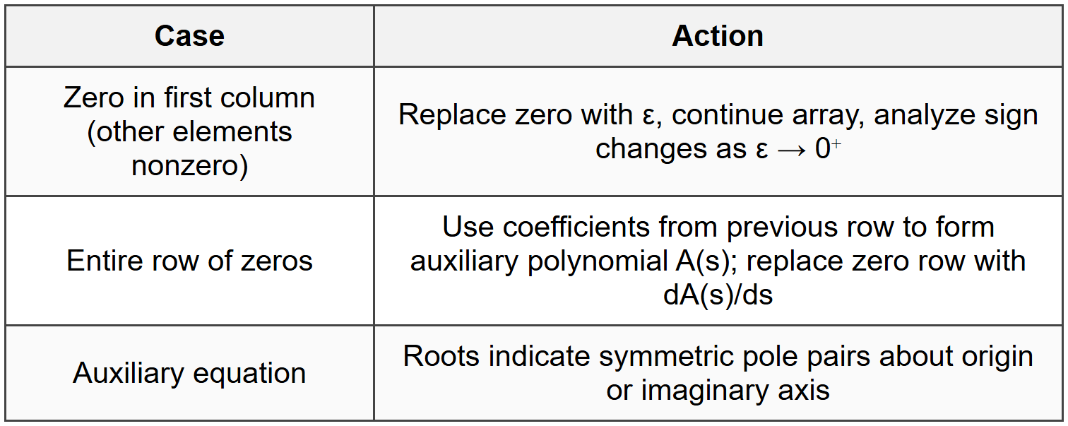
• Zero in first column: Replace with small ε > 0 and examine limit as ε → 0
• Entire row of zeros: Indicates poles on imaginary axis; form auxiliary equation from previous row

2.3 Special Cases

3. Root Locus Method

3.1 Root Locus Fundamentals

3.2 Root Locus Construction Rules

3.3 Gain Calculation on Root Locus

For point s₀ on locus: K = |∏(s₀ - zᵢ)|/|∏(s₀ - pⱼ)|

• Product of vector lengths from poles divided by product of vector lengths from zeros
• Use magnitude condition: K = 1/|G(s₀)H(s₀)|

4. Nyquist Stability Criterion

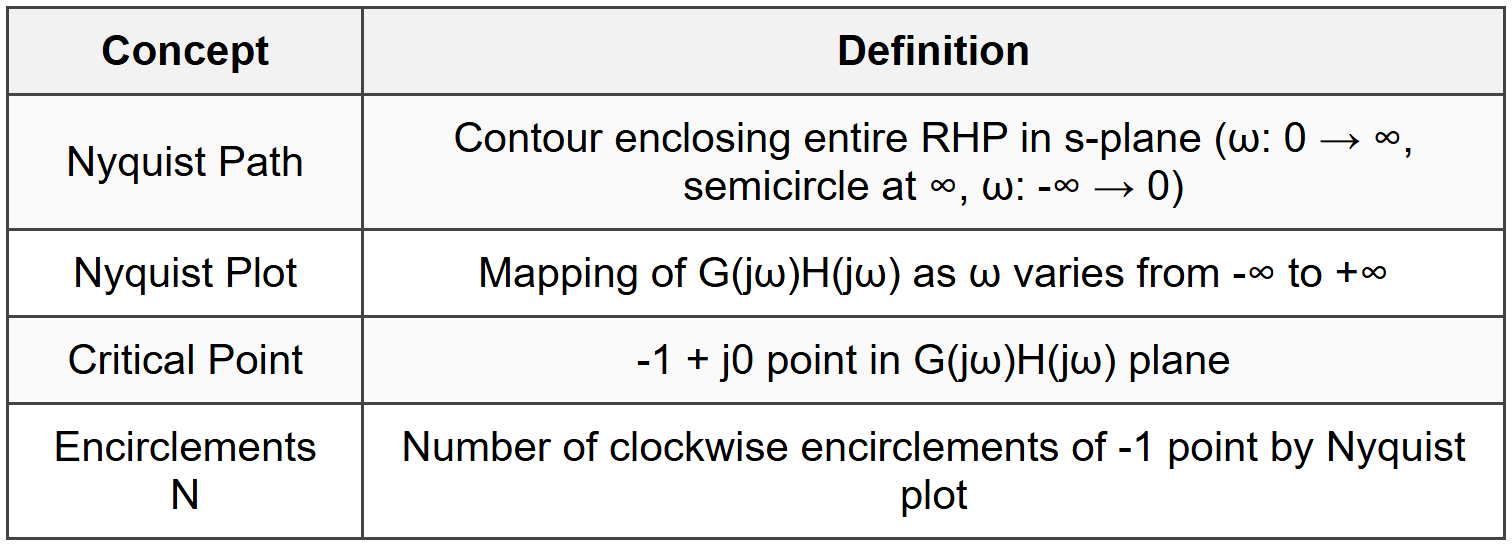
4.1 Nyquist Fundamentals

4.2 Nyquist Stability Criterion

Z = N + P

• Z = number of closed-loop poles in RHP (unstable poles)
• N = number of clockwise encirclements of -1 point
• P = number of open-loop poles in RHP
• For stability: Z = 0, therefore N = -P
• If P = 0 (open-loop stable): no encirclements of -1 for closed-loop stability
• Counterclockwise encirclements count as negative N

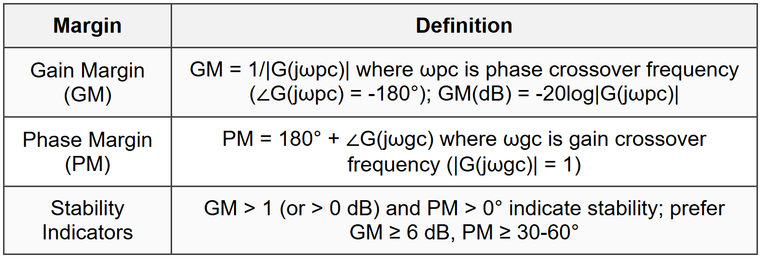
4.3 Gain and Phase Margins

4.4 Nyquist Plot Construction

• Start at ω = 0⁺: evaluate G(j0)H(j0)
• For poles/zeros at origin: plot includes semicircular arc at infinity
• Type 0: starts at finite positive real axis value
• Type 1: semicircle from -90° (ω = 0⁺) with radius → ∞
• Type 2: semicircle from -180° (ω = 0⁺) with radius → ∞
• Plot G(jω)H(jω) for ω: 0 → ∞, then mirror about real axis for ω: -∞ → 0
• End point as ω → ∞: approaches origin at angle -90°(n - m)

5. Bode Plot Stability Analysis

5.1 Bode Plot Basics

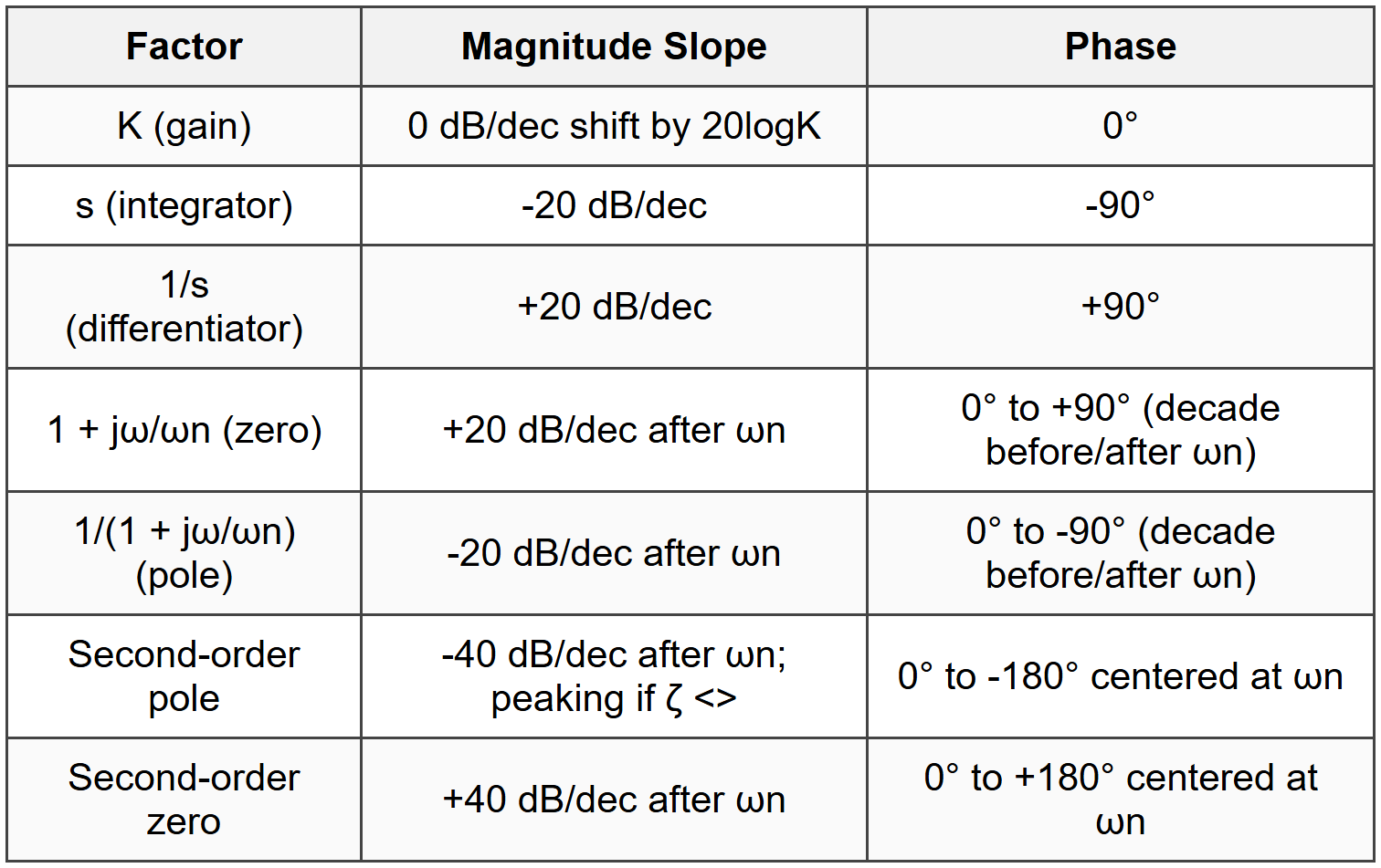
5.2 Standard Factor Contributions

5.3 Stability from Bode Plots

• System stable if PM > 0° and GM > 0 dB
• Read PM at gain crossover frequency: PM = 180° + ∠G(jωgc)
• Read GM at phase crossover frequency: GM(dB) = -20log|G(jωpc)|
• If phase never reaches -180°, GM = ∞
• Typical design targets: GM ≥ 6 dB, PM ≥ 30-60°
• Slope at gain crossover should be -20 dB/dec for good stability

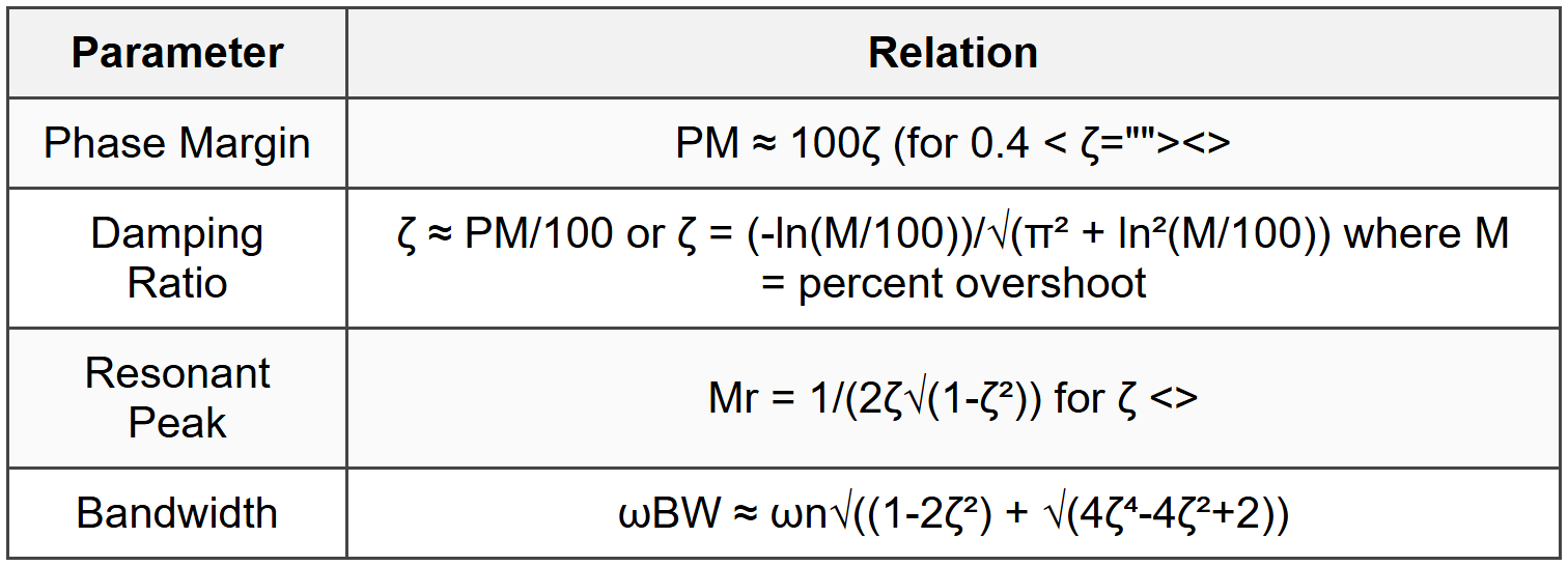
5.4 Second-Order System Approximations

6. State-Space Stability Analysis

6.1 State-Space Representation

ẋ = Ax + Bu; y = Cx + Du

• x: state vector (n × 1)
• A: system matrix (n × n)
• B: input matrix (n × m)
• C: output matrix (p × n)
• D: feedthrough matrix (p × m)

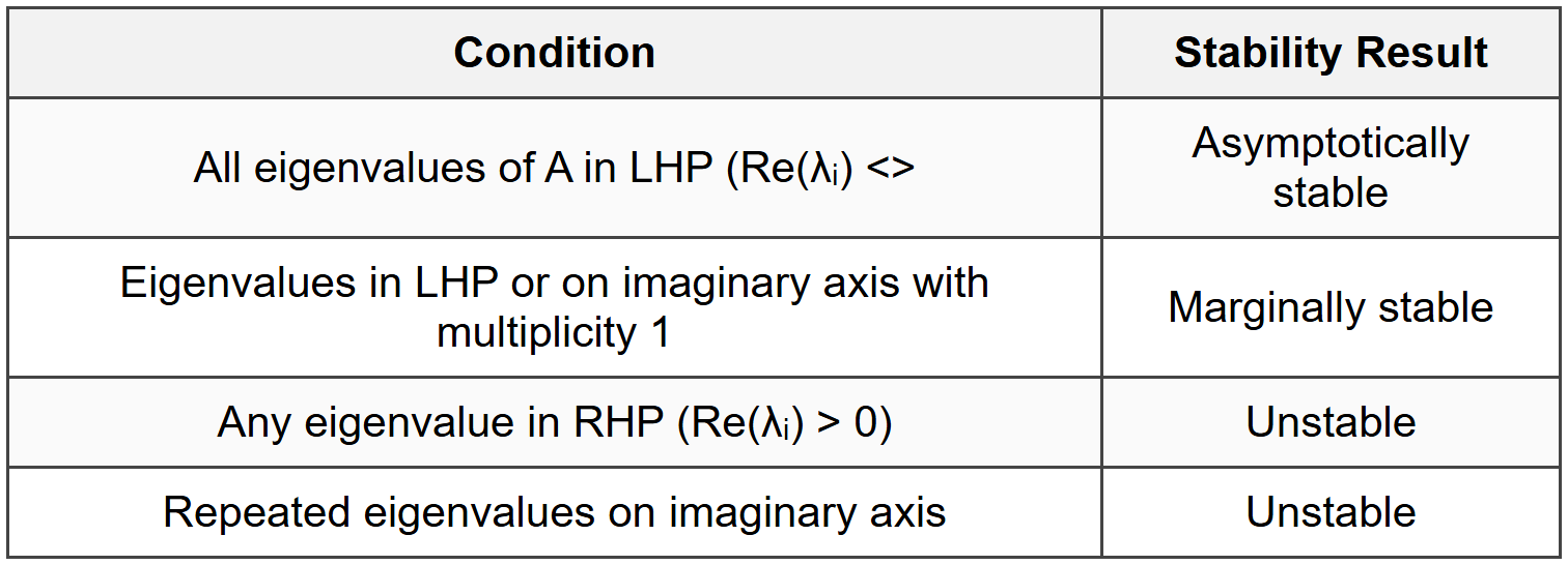
6.2 Eigenvalue-Based Stability

6.3 Lyapunov Stability Theory

6.3.1 Lyapunov Direct Method

• Find Lyapunov function V(x) > 0 for x ≠ 0, V(0) = 0
• If dV/dt = ∂V/∂x · ẋ < 0="" for="" x="" ≠="" 0,="" system="" is="" asymptotically="">
• If dV/dt ≤ 0, system is stable
• If dV/dt > 0, system is unstable
• Common choice: V(x) = xᵀPx where P is positive definite

6.3.2 Lyapunov Equation (Linear Systems)

AᵀP + PA = -Q

• If Q is positive definite and P is positive definite, system is asymptotically stable
• Common choice: Q = I (identity matrix)
• Solve for P; check if P is positive definite (all eigenvalues > 0 or all leading principal minors > 0)

6.4 Controllability and Observability

7. Discrete-Time Stability

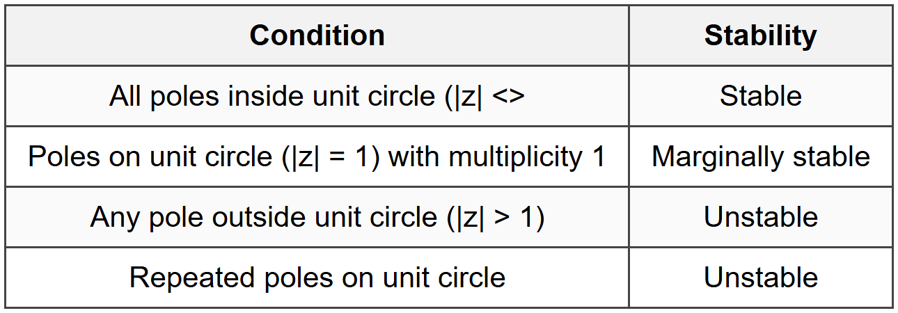
7.1 Z-Domain Stability

7.2 Jury Stability Test

For characteristic equation: a₀zⁿ + a₁zⁿ⁻¹ + ... + aₙ = 0

• Necessary conditions: P(1) > 0, (-1)ⁿP(-1) > 0, |aₙ| <>
• Form Jury table with 2n-3 rows alternating coefficients and computed values
• Sufficient condition: Elements in first column must satisfy magnitude conditions
• More complex than Routh-Hurwitz; often easier to use bilinear transformation

7.3 Bilinear Transformation (w-transform)

z = (1 + w)/(1 - w) or w = (z - 1)/(z + 1)

• Maps interior of unit circle in z-plane to LHP in w-plane
• After substitution, apply Routh-Hurwitz to polynomial in w
• System stable in z-domain if resulting w-domain system is stable

7.4 Discrete State-Space Stability

x[k+1] = Φx[k] + Γu[k]; y[k] = Cx[k] + Du[k]

• Φ: state transition matrix (discrete)
• Stability determined by eigenvalues of Φ
• All eigenvalues must satisfy |λᵢ| <>
• Discrete Lyapunov equation: ΦᵀPΦ - P = -Q

8. Relative Stability and Performance Metrics

8.1 Time-Domain Specifications

8.2 Steady-State Error Constants

8.3 System Type and Error

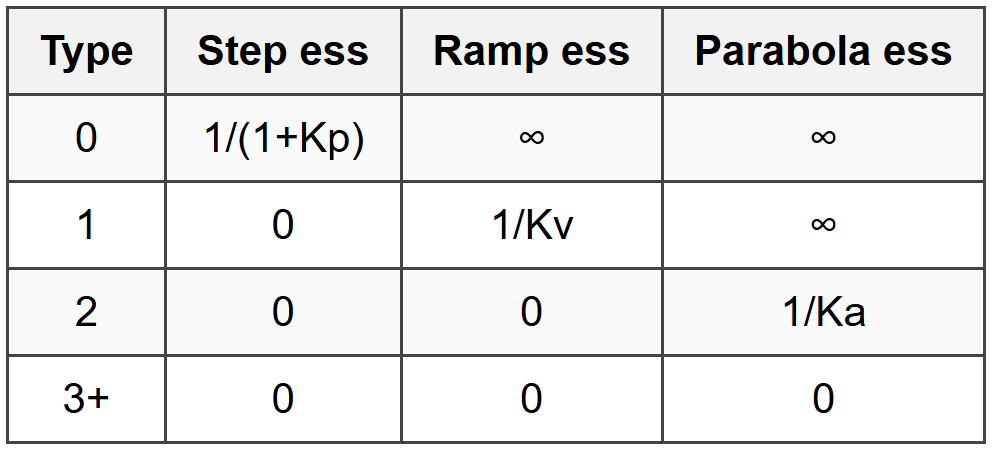
System type = number of poles at origin in open-loop transfer function G(s)H(s)

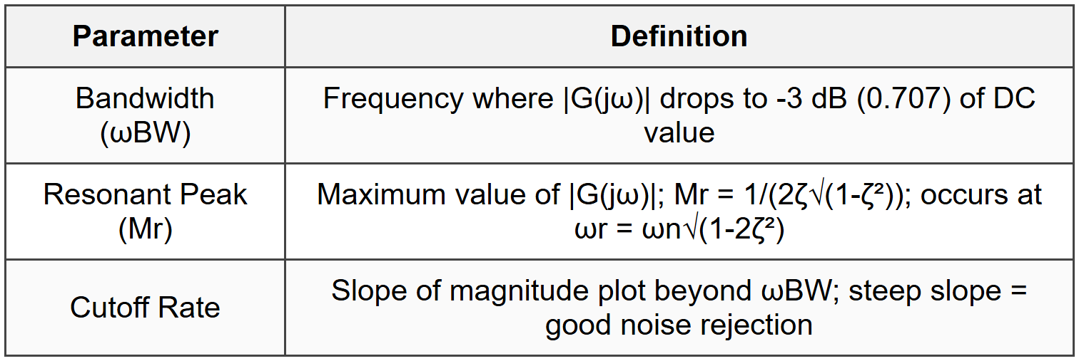
8.4 Frequency-Domain Performance

9. Advanced Stability Topics

9.1 Gain and Phase Margins from Root Locus

• Find K at imaginary axis crossing (use Routh-Hurwitz)
• Gain margin: ratio of K at instability to actual K
• Phase margin: angle from dominant pole to negative real axis (approximation)

9.2 Conditional Stability

• System stable for certain gain ranges but unstable outside those ranges
• Multiple crossings of -1 point on Nyquist plot
• Requires careful gain selection
• Bode plot shows multiple phase crossovers

9.3 Nichols Chart

• Plot of magnitude (dB) vs. phase of G(jω) on rectangular coordinates
• Contours of constant closed-loop magnitude and phase
• Read closed-loop frequency response directly
• Stability: curve must not enclose -1 point (0 dB, -180°)
• Gain and phase margins read directly from chart

9.4 Describing Function Analysis (Nonlinear Systems)

• Approximate nonlinearity by fundamental harmonic response
• N(A) = describing function, depends on input amplitude A
• Stability condition: -1/N(A) must not intersect G(jω)
• Used for limit cycle prediction in nonlinear systems
• Common nonlinearities: saturation, deadzone, relay, hysteresis

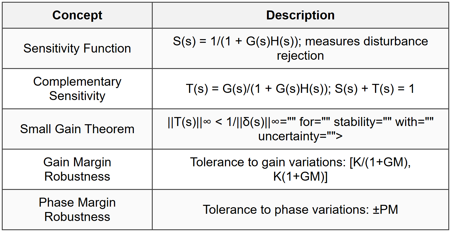
9.5 Robust Stability

10. Practical Stability Considerations

10.1 Design Guidelines

• Phase margin: 30-60° (45° optimal for good balance)
• Gain margin: ≥6 dB (factor of 2)
• Crossover frequency should have slope of -20 dB/dec
• Maximize bandwidth while maintaining adequate margins
• Place dominant poles to achieve desired transient response
• Keep nondominant poles at least 5-10 times farther from imaginary axis

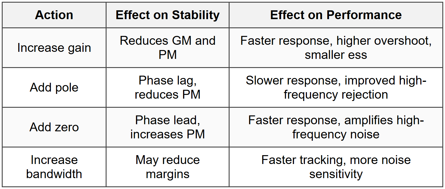
10.2 Stability Margins Trade-offs

10.3 Common Stability Issues

• Time delays: e^(-sτ) adds phase lag; approximations: Padé, Taylor series
• Saturation: nonlinearity can cause limit cycles or instability in large-signal operation
• Sensor noise: high gain amplifies noise; requires filtering
• Unmodeled dynamics: high-frequency poles/zeros can destabilize system
• Parameter variations: use robust design to handle uncertainty

10.4 Stability Testing Procedure

1. Find characteristic equation: 1 + KG(s)H(s) = 0
2. Check necessary conditions: all coefficients present and same sign
3. Apply Routh-Hurwitz or plot root locus
4. Verify GM and PM from Bode or Nyquist plot
5. Calculate time-domain specifications if needed
6. Check robustness to parameter variations
7. Simulate to verify analysis and check for nonlinear effects