Cheatsheet: Signals And Systems

1. Signal Classification

1.1 Continuous-Time vs Discrete-Time

1.2 Analog vs Digital

1.3 Periodic vs Aperiodic

1.4 Even vs Odd Signals

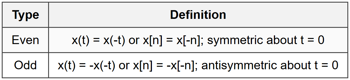
• Any signal can be decomposed: x(t) = xₑ(t) + xₒ(t)
• Even part: xₑ(t) = ½[x(t) + x(-t)]
• Odd part: xₒ(t) = ½[x(t) - x(-t)]

1.5 Energy vs Power Signals

• Energy and power signals are mutually exclusive
• Periodic signals are power signals
• Finite-duration signals are energy signals

1.6 Deterministic vs Random

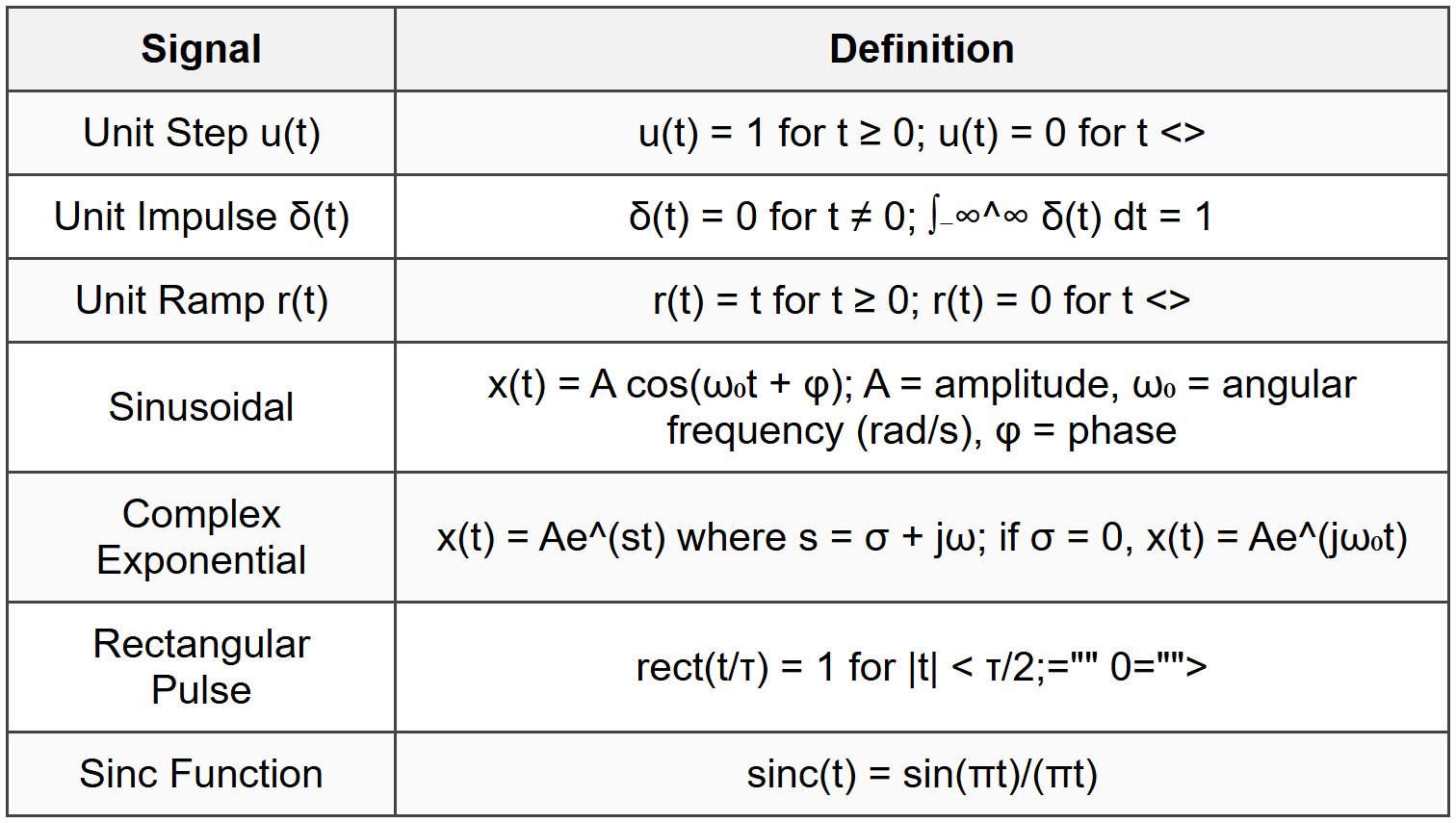
2. Basic Signals

2.1 Continuous-Time Signals

2.2 Discrete-Time Signals

2.3 Impulse Properties

• Sifting property: ∫₋∞^∞ x(t)δ(t - t₀) dt = x(t₀)
• Discrete sifting: Σₙ₌₋∞^∞ x[n]δ[n - n₀] = x[n₀]
• Derivative of step: δ(t) = du(t)/dt
• Discrete step relation: δ[n] = u[n] - u[n-1]
• Scaling: δ(at) = (1/|a|)δ(t)

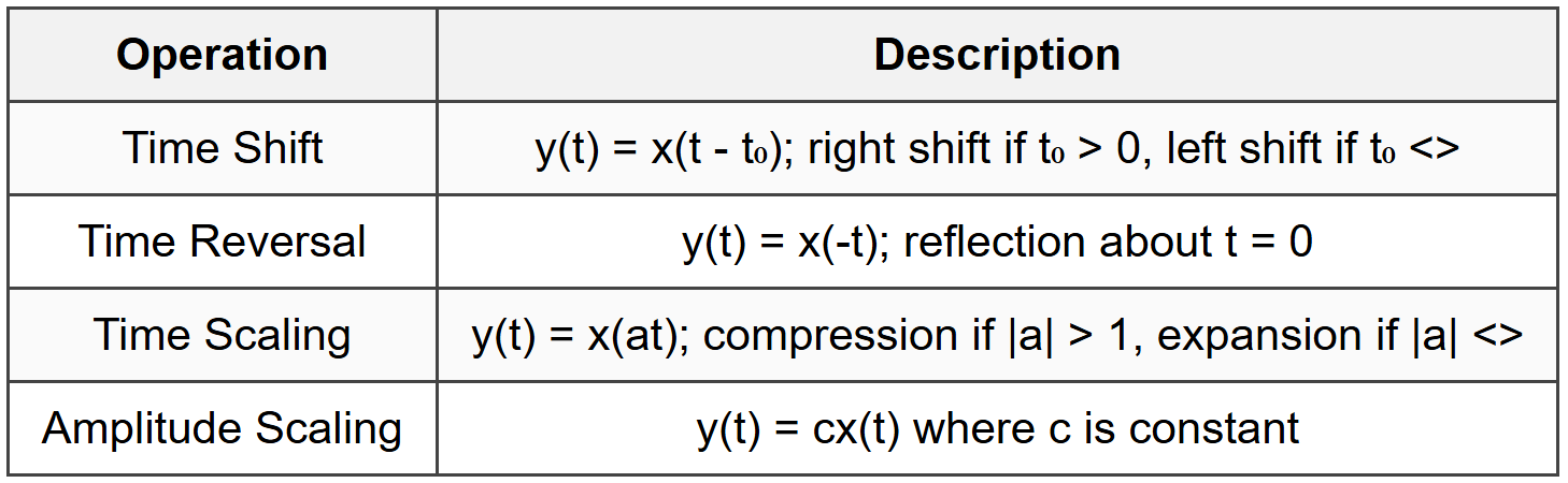
3. Signal Operations

3.1 Time-Domain Operations

3.2 Order of Operations

• For y(t) = x(at - b): 1) time scaling by a, 2) time shift by b/a
• For y(t) = x(at + b): 1) time scaling by a, 2) time shift by -b/a
• Alternative: 1) shift by b, 2) scale by a (different result)

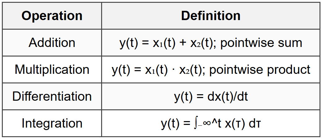
3.3 Arithmetic Operations

4. System Properties

4.1 Linearity

• System is linear if: T[ax₁(t) + bx₂(t)] = aT[x₁(t)] + bT[x₂(t)]
• Satisfies additivity: T[x₁(t) + x₂(t)] = T[x₁(t)] + T[x₂(t)]
• Satisfies homogeneity: T[ax(t)] = aT[x(t)]

4.2 Time-Invariance

• If x(t) → y(t), then x(t - t₀) → y(t - t₀) for all t₀
• System characteristics do not change with time

4.3 Causality

• Output at time t₀ depends only on input for t ≤ t₀
• Non-anticipative system
• For h(t): causal if h(t) = 0 for t <>
• For h[n]: causal if h[n] = 0 for n <>

4.4 Stability (BIBO)

• Bounded-Input Bounded-Output stable
• If |x(t)| < m="">< ∞,="" then="" |y(t)|="">< n=""><>
• CT condition: ∫₋∞^∞ |h(t)| dt <>
• DT condition: Σₙ₌₋∞^∞ |h[n]| <>

4.5 Memory

4.6 Invertibility

• Inverse system exists such that cascading gives identity
• Distinct inputs produce distinct outputs

5. LTI Systems

5.1 Convolution

5.2 Convolution Properties

• Commutative: x(t) * h(t) = h(t) * x(t)
• Associative: [x(t) * h₁(t)] * h₂(t) = x(t) * [h₁(t) * h₂(t)]
• Distributive: x(t) * [h₁(t) + h₂(t)] = x(t) * h₁(t) + x(t) * h₂(t)
• Identity: x(t) * δ(t) = x(t)
• Shift property: x(t) * δ(t - t₀) = x(t - t₀)

5.3 Impulse Response

• h(t) = T[δ(t)]; characterizes LTI system completely
• Output: y(t) = x(t) * h(t)
• Parallel connection: h(t) = h₁(t) + h₂(t)
• Series connection: h(t) = h₁(t) * h₂(t)

5.4 Step Response

• s(t) = ∫₋∞^t h(τ) dτ = h(t) * u(t)
• h(t) = ds(t)/dt
• s[n] = Σₖ₌₋∞^n h[k] = h[n] * u[n]
• h[n] = s[n] - s[n-1]

6. Fourier Analysis

6.1 Fourier Series (Continuous-Time)

• aₖ = (1/T) ∫₀^T x(t)cos(kω₀t) dt; k ≥ 0
• bₖ = (1/T) ∫₀^T x(t)sin(kω₀t) dt; k ≥ 1
• a₀ = (1/T) ∫₀^T x(t) dt (DC component)

6.2 Fourier Series (Discrete-Time)

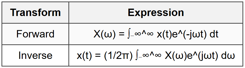
6.3 Fourier Transform (Continuous-Time)

6.4 Fourier Transform Properties

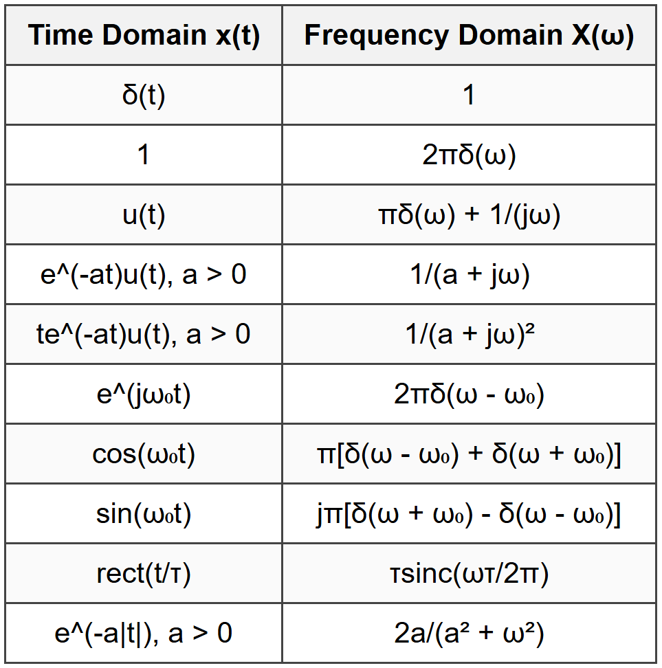
6.5 Common Fourier Transform Pairs

6.6 Discrete-Time Fourier Transform (DTFT)

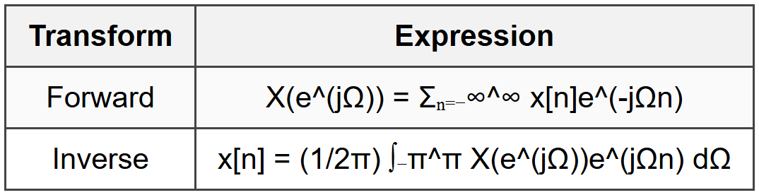
• X(e^(jΩ)) is periodic with period 2π
• Ω is discrete-time frequency in radians

6.7 Frequency Response

• H(ω) = Y(ω)/X(ω) = ℱ{h(t)}
• y(t) = x(t) * h(t) ↔ Y(ω) = X(ω)H(ω)
• |H(ω)| = magnitude response
• ∠H(ω) = phase response

7. Laplace Transform

7.1 Definitions

• s = σ + jω (complex frequency)
• Region of Convergence (ROC) specifies values of s for which X(s) converges

7.2 ROC Properties

• ROC consists of vertical strips in s-plane
• For rational X(s), ROC bounded by poles
• Right-sided signal: ROC is Re{s} > σ₀
• Left-sided signal: ROC is Re{s} <>
• Two-sided signal: ROC is σ₁ < re{s}=""><>
• Finite duration: ROC is entire s-plane
• Causal signal: ROC is to right of rightmost pole

7.3 Laplace Transform Properties

7.4 Common Laplace Transform Pairs

7.5 Transfer Function

• H(s) = Y(s)/X(s) with zero initial conditions
• H(s) = ℒ{h(t)}
• Poles: roots of denominator (make H(s) → ∞)
• Zeros: roots of numerator (make H(s) = 0)
• System stable if all poles in left half-plane (Re{s} <>

7.6 Partial Fraction Expansion

• For proper rational X(s) = N(s)/D(s) where degree(N) <>
• Simple poles: X(s) = Σᵢ Aᵢ/(s - pᵢ); Aᵢ = [(s - pᵢ)X(s)]|ₛ₌ₚᵢ
• Repeated poles (order r): additional terms with (s - pᵢ)^k in denominator
• Complex conjugate poles: combine terms for real time-domain result

8. Z-Transform

8.1 Definitions

• z = re^(jΩ) (complex variable)
• ROC specifies values of z for which X(z) converges

8.2 ROC Properties

• ROC consists of rings or disks in z-plane
• For rational X(z), ROC bounded by poles
• Right-sided sequence: ROC is |z| > r₀
• Left-sided sequence: ROC is |z| <>
• Two-sided sequence: ROC is r₁ < |z|=""><>
• Finite duration: ROC is entire z-plane (except possibly z = 0 or z = ∞)
• Causal sequence: ROC is exterior of circle beyond outermost pole

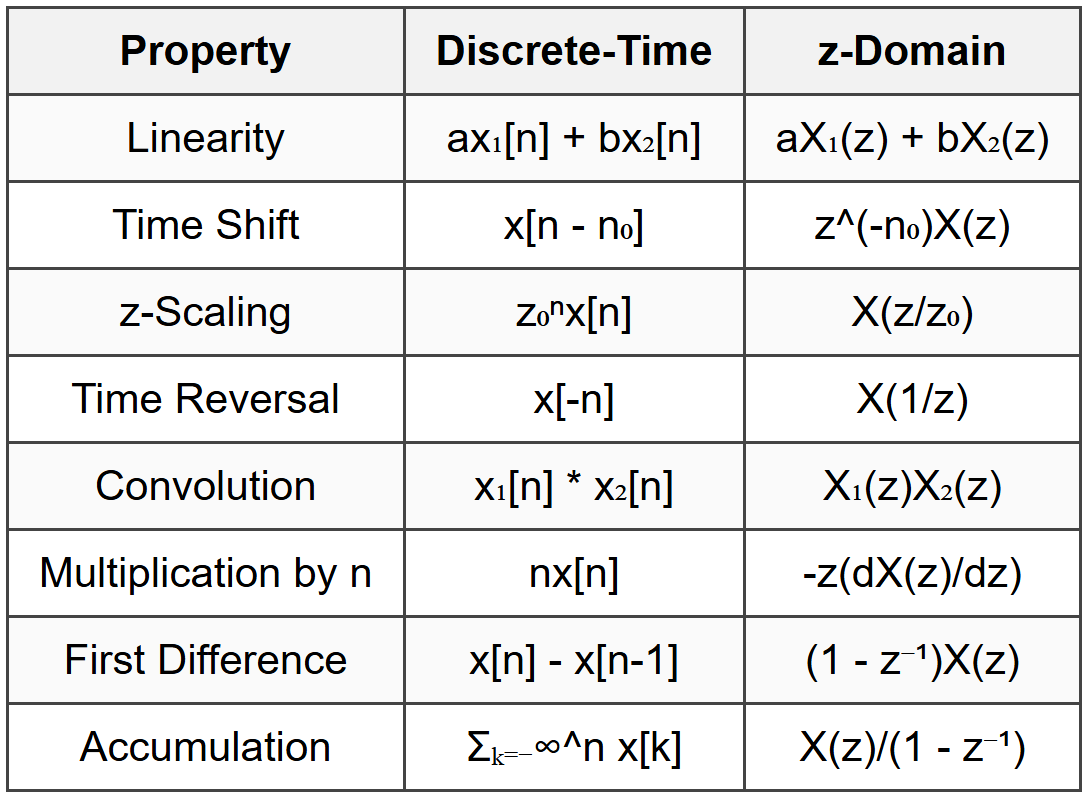
8.3 Z-Transform Properties

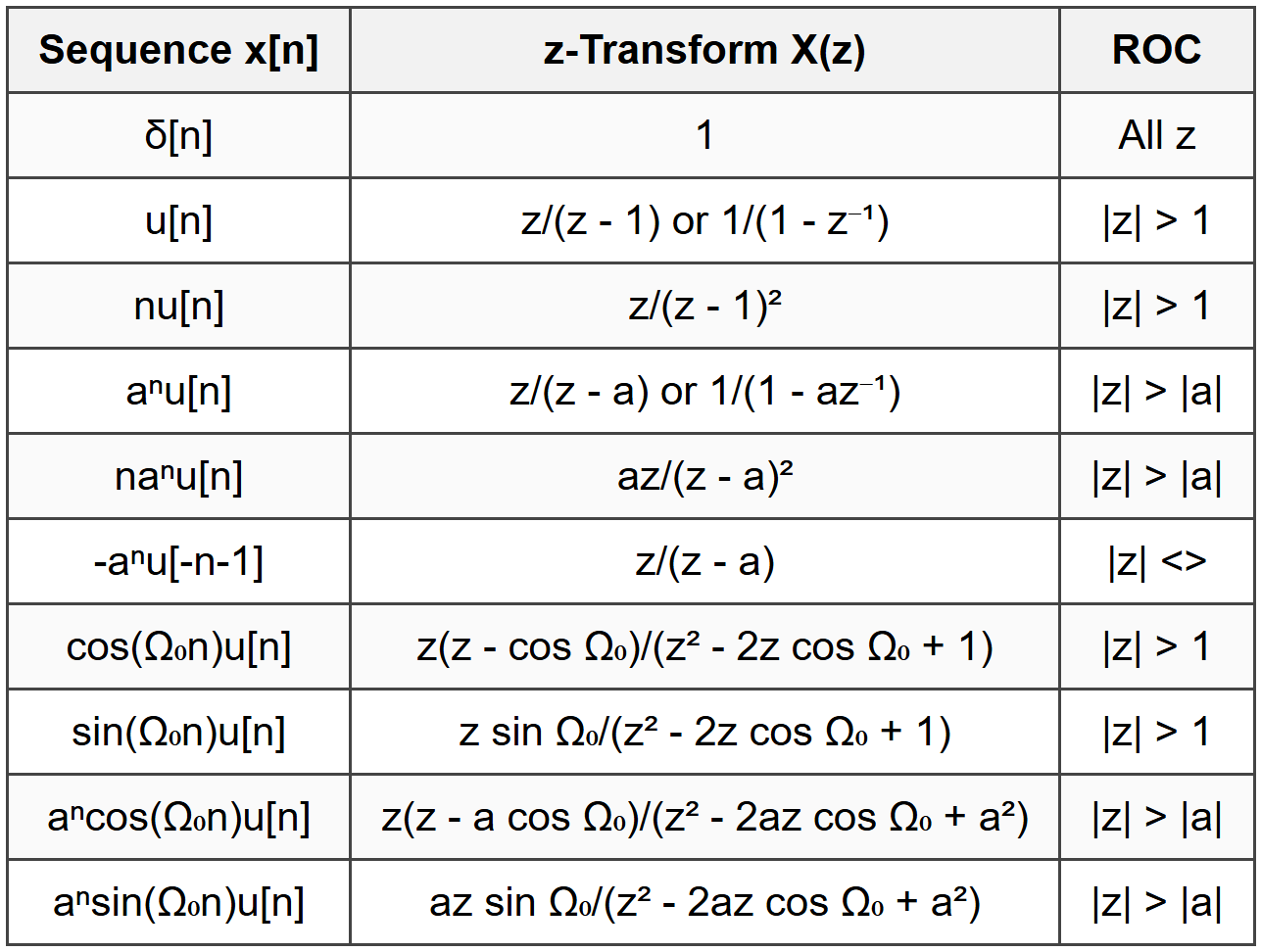
8.4 Common Z-Transform Pairs

8.5 Transfer Function

• H(z) = Y(z)/X(z) with zero initial conditions
• H(z) = ℤ{h[n]}
• Poles: roots of denominator
• Zeros: roots of numerator
• System stable if all poles inside unit circle (|z| <>

8.6 Relation to DTFT

• DTFT is Z-transform evaluated on unit circle: X(e^(jΩ)) = X(z)|_(z=e^(jΩ))
• DTFT exists if ROC includes unit circle

9. Sampling and Reconstruction

9.1 Sampling Theorem

• Nyquist-Shannon sampling theorem
• Bandlimited signal with maximum frequency fₘ can be reconstructed if sampling frequency fₛ ≥ 2fₘ
• Nyquist rate: fₙ = 2fₘ (minimum sampling rate)
• Nyquist frequency: fₙ/2 (maximum frequency that can be represented)
• ωₛ ≥ 2ωₘ for angular frequencies

9.2 Aliasing

• Occurs when fₛ <>
• High-frequency components appear as lower frequencies
• Frequency folding about fₛ/2
• Prevented by anti-aliasing filter before sampling

9.3 Ideal Sampling

• xₚ(t) = x(t) · Σₙ₌₋∞^∞ δ(t - nT) where T = 1/fₛ
• Xₚ(ω) = (1/T) Σₖ₌₋∞^∞ X(ω - kωₛ) where ωₛ = 2π/T
• Spectrum repeats every ωₛ

9.4 Reconstruction

• Ideal reconstruction: x(t) = Σₙ₌₋∞^∞ x(nT)sinc[(t - nT)/T]
• Ideal lowpass filter: H(ω) = T for |ω| < ωₛ/2;="" 0="">
• Zero-order hold (ZOH): piecewise constant between samples

10. Digital Filter Structures

10.1 Difference Equations

• General form: Σₖ₌₀^N aₖy[n-k] = Σₖ₌₀^M bₖx[n-k]
• Causal: y[n] = (1/a₀)[Σₖ₌₀^M bₖx[n-k] - Σₖ₌₁^N aₖy[n-k]]
• Order: max(M, N)

10.2 FIR vs IIR Filters

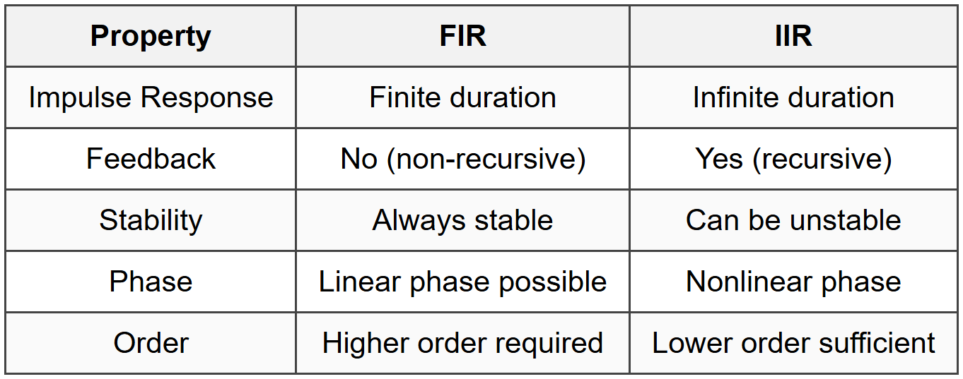
10.3 FIR Filter

• y[n] = Σₖ₌₀^(M-1) bₖx[n-k]
• H(z) = Σₖ₌₀^(M-1) bₖz^(-k)
• All poles at z = 0
• M coefficients, order M-1

10.4 IIR Filter

• y[n] = Σₖ₌₀^M bₖx[n-k] - Σₖ₌₁^N aₖy[n-k]
• H(z) = (Σₖ₌₀^M bₖz^(-k))/(1 + Σₖ₌₁^N aₖz^(-k))
• Poles not restricted to origin
• Requires stability check

11. Filter Design

11.1 Filter Specifications

11.2 Analog Filter Prototypes

11.3 Filter Types

• Lowpass: passes frequencies below cutoff
• Highpass: passes frequencies above cutoff
• Bandpass: passes frequencies within band [ω₁, ω₂]
• Bandstop (notch): attenuates frequencies within band

11.4 Bilinear Transformation

• Maps s-plane to z-plane: s = (2/T)[(z - 1)/(z + 1)]
• z = (1 + sT/2)/(1 - sT/2)
• Maps jω axis to unit circle
• Left half s-plane maps to interior of unit circle
• Frequency warping: Ω = (2/T)tan(ωT/2)
• Prewarping: compensate by designing at ω' = (2/T)tan(ωT/2)

12. State-Space Analysis

12.1 State Equations

• x = state vector (n × 1)
• u = input vector (p × 1)
• y = output vector (q × 1)
• A = system matrix (n × n)
• B = input matrix (n × p)
• C = output matrix (q × n)
• D = feedthrough matrix (q × p)

12.2 State-Space to Transfer Function

• H(s) = C(sI - A)⁻¹B + D
• H(z) = C(zI - A)⁻¹B + D
• Poles: eigenvalues of A (roots of det(sI - A) = 0)

12.3 Solutions

• CT: x(t) = e^(At)x(0) + ∫₀^t e^(A(t-τ))Bu(τ) dτ
• DT: x[n] = Aⁿx[0] + Σₖ₌₀^(n-1) A^(n-1-k)Bu[k]
• State transition matrix: Φ(t) = e^(At) or Φ[n] = Aⁿ

12.4 Controllability and Observability