Cheatsheet: Process Control

1. Fundamentals of Process Control

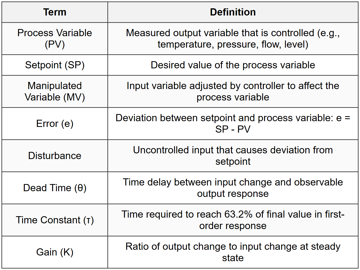
1.1 Basic Definitions

1.2 Control System Components

• Sensor/Transmitter: Measures process variable and converts to signal
• Controller: Compares PV to SP and determines control action
• Final Control Element: Executes controller output (valve, damper, motor)
• Process: System being controlled

1.3 Control Loop Types

2. Transfer Functions and Dynamic Response

2.1 Laplace Transform Basics

2.2 Standard Transfer Functions

2.2.1 First-Order System

• G(s) = K/(τs + 1)
• Step response: y(t) = K[1 - e^-t/τ]
• Settling time (95%): t_s = 3τ; (98%): t_s = 4τ

2.2.2 Second-Order System

• G(s) = K/(τ²s² + 2ζτs + 1)
• ζ = damping ratio; ζ < 1="" (underdamped),="" ζ="1" (critically="" damped),="" ζ=""> 1 (overdamped)
• Natural frequency: ω_n = 1/τ
• Overshoot (for ζ < 1):="" os="">^{-πζ/√(1-ζ²)} × 100%
• Rise time: t_r ≈ (1.8/ω_n) for ζ = 0.5

2.2.3 Dead Time (Transport Lag)

• G(s) = e^-θs
• First-order plus dead time (FOPDT): G(s) = Ke^-θs/(τs + 1)

2.3 Block Diagram Algebra

3. PID Control

3.1 PID Controller Equation

• Time domain: u(t) = K_c[e(t) + (1/τ_I)∫e(t)dt + τ_D(de/dt)]
• Transfer function: G_c(s) = K_c[1 + 1/(τ_Is) + τ_Ds]
• Alternative form: G_c(s) = K_c + K_I/s + K_Ds
• K_I = K_c/τ_I; K_D = K_cτ_D

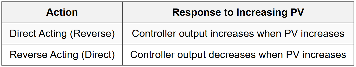
3.2 Controller Actions

3.3 Effect of Controller Parameters

3.4 Controller Tuning Methods

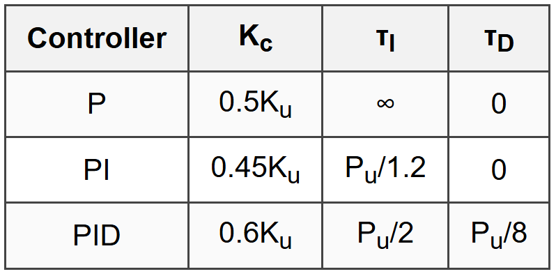
3.4.1 Ziegler-Nichols Closed Loop (Ultimate Gain Method)

• Set τ_I = ∞, τ_D = 0; increase K_c until sustained oscillation
• K_u = ultimate gain; P_u = period of oscillation

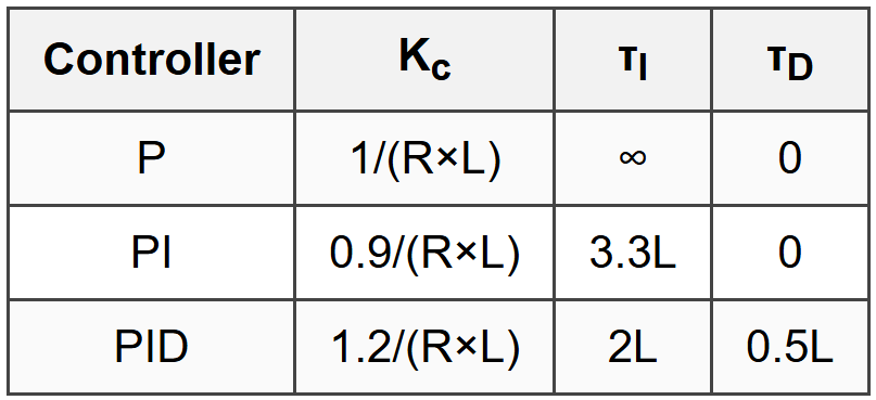
3.4.2 Ziegler-Nichols Open Loop (Reaction Curve Method)

• Apply step change to MV; measure S = slope at inflection point, θ = dead time, K = process gain
• Alternative: R = S/K; L = θ

3.4.3 Cohen-Coon Method

• For FOPDT model: G(s) = Ke^-θs/(τs + 1)
• Define: α = θ/τ (dead time to time constant ratio)

3.4.4 IMC (Internal Model Control) Tuning

• For FOPDT: K_c = τ/[K(θ + λ)]; τ_I = τ; τ_D = 0
• λ = desired closed-loop time constant (tuning parameter); larger λ = more conservative

4. Stability Analysis

4.1 Routh-Hurwitz Stability Criterion

• Characteristic equation: a_nsⁿ + a_n-1s^n-1 + ... + a₁s + a₀ = 0
• Construct Routh array; system stable if all elements in first column have same sign
• Number of sign changes = number of roots in right half-plane (unstable)

4.2 Bode Stability Criterion

4.3 Root Locus Method

• Plots roots of characteristic equation as parameter (K_c) varies
• System stable when all roots in left half of s-plane
• Roots on imaginary axis indicate marginal stability

5. Advanced Control Strategies

5.1 Cascade Control

• Primary (master) controller output sets setpoint for secondary (slave) controller
• Secondary loop responds faster to disturbances
• Tune secondary controller first, then primary
• Secondary loop time constant should be 3-5 times faster than primary

5.2 Feedforward Control

• Measures disturbance and compensates before affecting PV
• Controller: G_FF(s) = -G_d(s)/G_p(s)
• G_d = disturbance transfer function; G_p = process transfer function
• Often combined with feedback control

5.3 Ratio Control

• Maintains ratio R = Flow A / Flow B
• Wild stream (uncontrolled flow) measured; captive stream manipulated
• Ratio setpoint adjusted to maintain desired proportion

5.4 Split-Range Control

• Single controller output operates two or more final control elements
• Each valve active over different ranges of controller output
• Example: 0-50% opens cooling valve; 50-100% opens heating valve

5.5 Override (Selective) Control

• Multiple controllers; selector chooses which controller output to use
• Low selector: chooses minimum signal
• High selector: chooses maximum signal
• Used for constraint control and safety

5.6 Model Predictive Control (MPC)

• Uses dynamic process model to predict future behavior
• Optimization performed at each time step over prediction horizon
• Handles multivariable systems and constraints
• Control horizon < prediction="">

6. Process Dynamics and Identification

6.1 Process Reaction Curve

• Open-loop step test to characterize process dynamics
• Graphical method: draw tangent at inflection point
• Dead time θ = time intercept; time constant τ = time to 63.2% of final value
• Process gain K = Δy/Δu (steady state)

6.2 Self-Regulating vs. Integrating Processes

6.3 Inverse Response

• Initial response in opposite direction to final response
• Right-half-plane zero in transfer function
• Requires slow controller tuning to avoid instability

7. Control Valve Sizing and Characteristics

7.1 Valve Flow Equation

• Q = C_v√(ΔP/G_f) for liquids
• Q = flow (gpm); C_v = valve coefficient; ΔP = pressure drop (psi); G_f = specific gravity
• For gases: Q = C_vP₁√(x/G_gT₁) with corrections for x = ΔP/P₁

7.2 Inherent Valve Characteristics

7.3 Installed Characteristics

• Actual flow vs. stroke under operating conditions
• Affected by system pressure drop distribution
• Equal percentage valve becomes more linear when installed

7.4 Valve Action

8. Controller Action and Loop Configuration

8.1 Controller Action Selection

8.2 Overall Loop Gain

• K_OL = K_c × K_v × K_p × K_m
• K_c = controller gain; K_v = valve gain; K_p = process gain; K_m = measurement gain
• For stability: K_OL must be negative (closed loop with negative feedback)

8.3 Pairing Variables in Multivariable Systems

• Relative Gain Array (RGA): λ_ij = (∂y_i/∂u_j)_{other loops open} / (∂y_i/∂u_j)_{other loops closed}
• Pair variables where λ_ij closest to 1.0
• Avoid pairing where λ_ij < 0="" (interaction="" causes="">

9. Common Process Control Applications

9.1 Level Control

• Averaging level control: loose control (large τ_I) to smooth flow variations
• Tight level control: fast response for precise control
• Integrating process: requires proportional or PI control only

9.2 Flow Control

• Fast process dynamics; use PI control with small τ_I
• Square root compensation needed for differential pressure flow measurement
• Flow control often used as secondary loop in cascade

9.3 Pressure Control

• Gas systems: fast response, potential for oscillation
• Liquid systems: slower, more stable
• Often use wide proportional band to prevent valve chattering

9.4 Temperature Control

• Large time constants and dead time; use PID control
• Heating/cooling systems benefit from cascade control
• Thermal processes often have long settling times

9.5 Distillation Column Control

• Fix 5 degrees of freedom: feed flow (external), reflux, distillate, bottoms, heat input
• Material balance control: L/D or V/B ratio
• Energy balance control: reflux ratio or boilup ratio
• Dual composition control: control both top and bottom product quality

9.6 Heat Exchanger Control

• Manipulate hot or cold stream flow rate
• Cascade: temperature controller sets flow controller setpoint
• Bypass control: split cold stream around exchanger

10. Performance Metrics

10.1 Time-Domain Performance Criteria

10.2 Offset

• Steady-state error between setpoint and process variable
• Proportional control has offset; PI and PID eliminate offset
• Offset = 1/(1 + K_cK_p) for P control with unit step disturbance

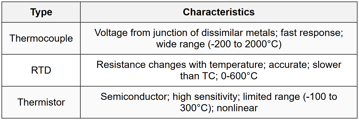
11. Instrumentation and Sensors

11.1 Temperature Sensors

11.2 Pressure Sensors

• Bourdon tube: mechanical deflection; 0-100,000 psi
• Diaphragm: pressure causes deflection measured capacitively or with strain gauge
• Piezoelectric: generates voltage under pressure; dynamic measurements

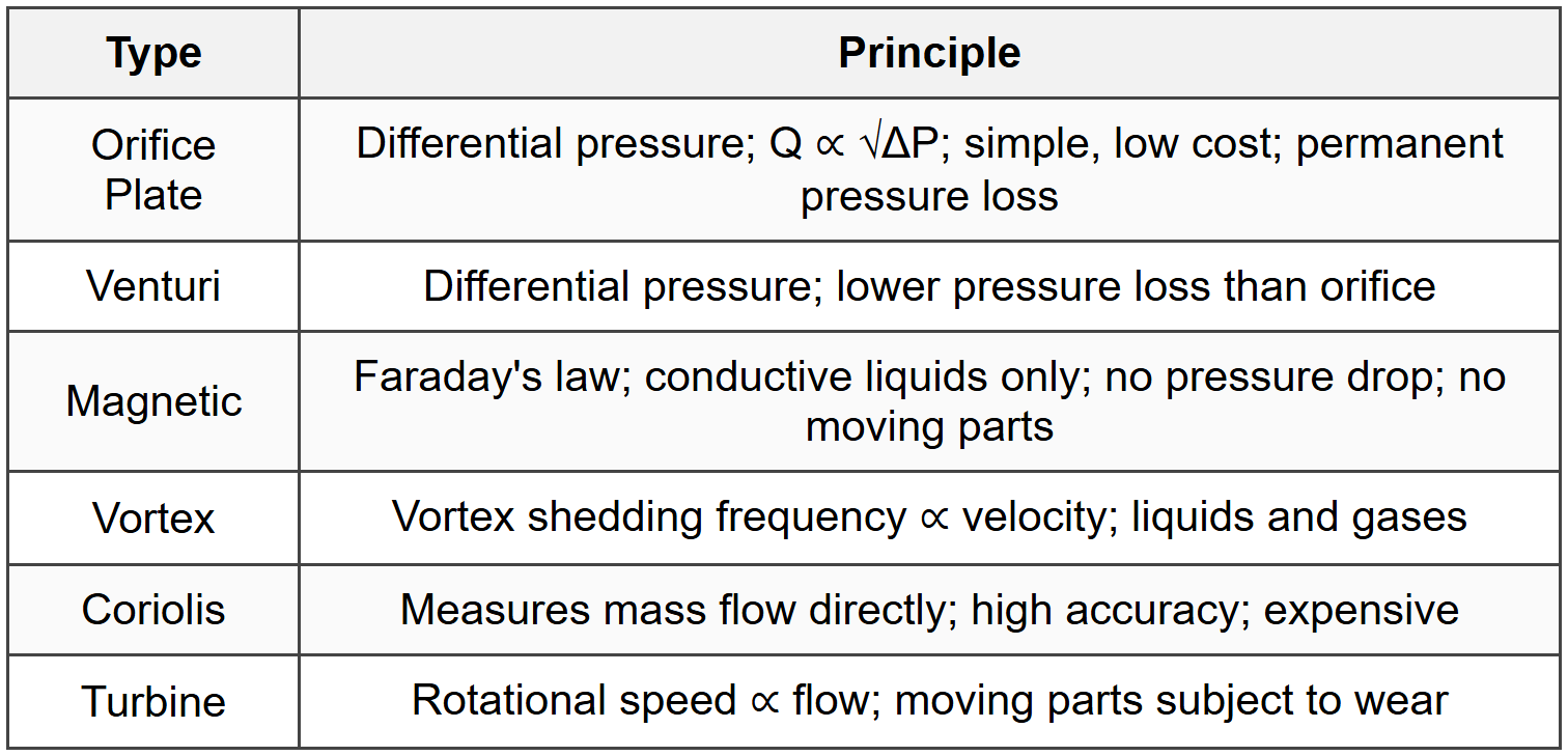
11.3 Flow Measurement

11.4 Level Measurement

• Differential pressure: ΔP = ρgh; affected by density changes
• Float: mechanical; simple, reliable
• Capacitance: dielectric between plates changes with level
• Ultrasonic: time-of-flight measurement; non-contact
• Radar: microwave reflection; handles vapor, foam, turbulence

11.5 Signal Standards

12. Frequency Response

12.1 Bode Plot Basics

• Magnitude plot: 20 log₁₀|G(jω)| vs. log ω (dB vs. frequency)
• Phase plot: ∠G(jω) vs. log ω (degrees vs. frequency)
• ω = frequency (rad/time)

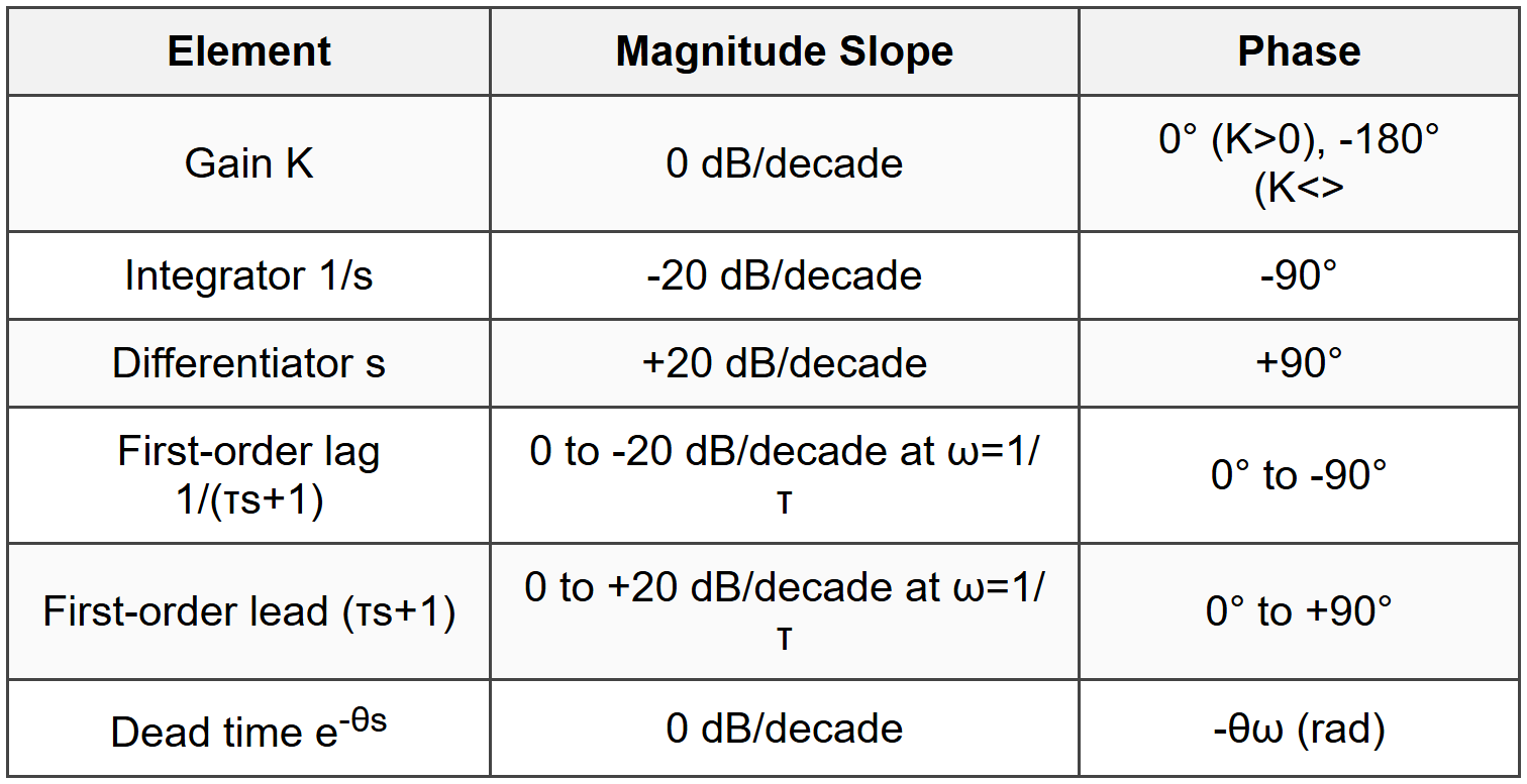
12.2 Common Transfer Function Elements

12.3 Bandwidth

• Frequency range where |G(jω)| > -3 dB (70.7% of DC gain)
• Wider bandwidth = faster response