Pump & system curves (basic conceptual)

This topic covers how pumps interact with piping systems through graphical analysis of pump curves and system curves. Understanding the operating point where these curves intersect is critical for solving FE exam problems involving pump selection, flow determination, and system performance prediction.

Core Concepts

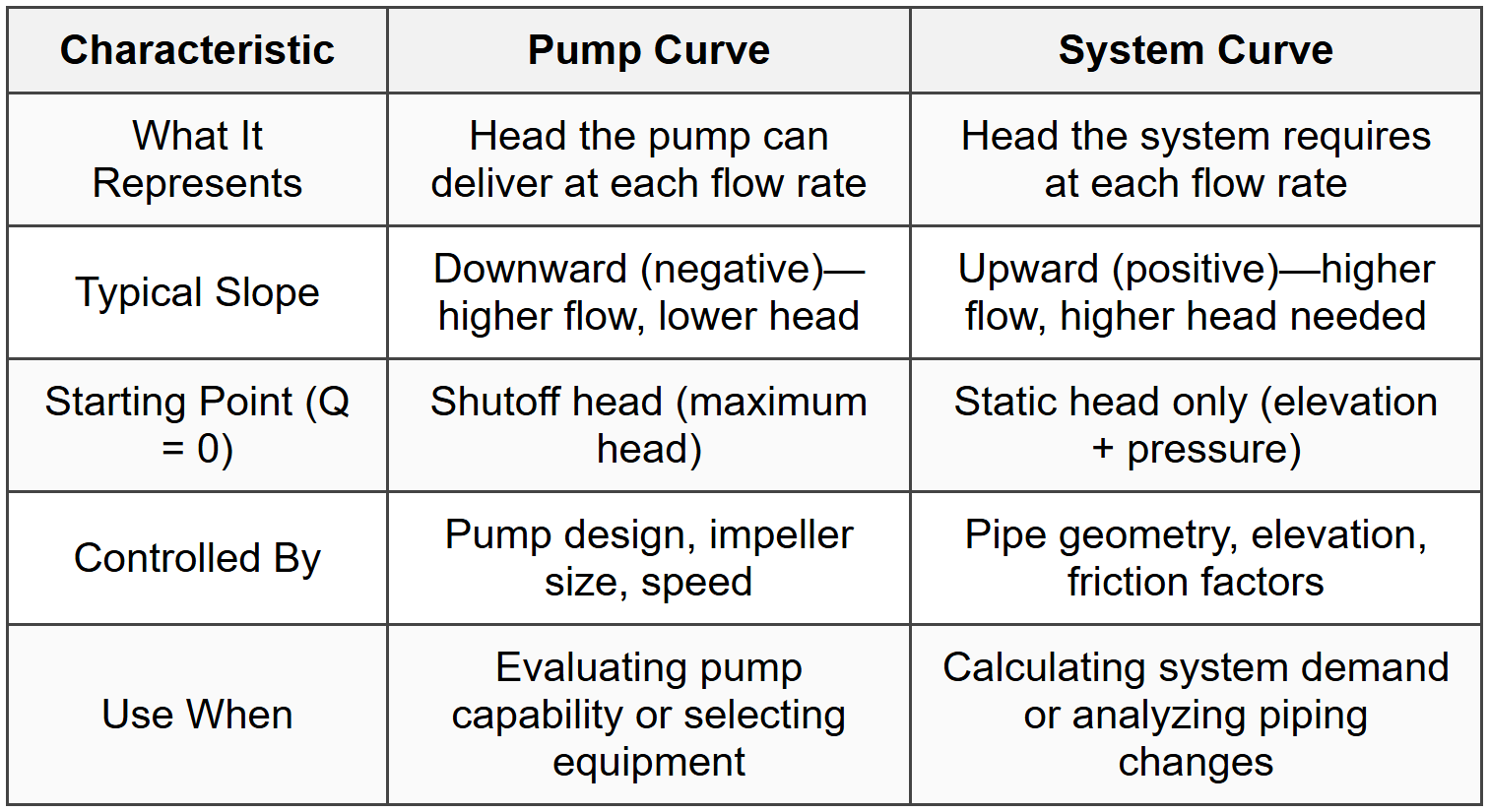
Pump Curve (Pump Characteristic Curve)

A pump curve shows the relationship between the head (pressure) a pump can deliver and the flow rate it produces at a constant speed. The pump generates maximum head at zero flow (shutoff head) and progressively less head as flow increases. This inverse relationship exists because energy losses within the pump increase with flow rate.

• The curve is typically provided by the pump manufacturer for a specific impeller diameter and rotational speed
• Head is measured in feet or meters of fluid column
• Flow rate is measured in gallons per minute (gpm), cubic feet per second (cfs), or liters per second (L/s)
• The curve slopes downward from left to right-higher flow means lower head output
• Peak efficiency occurs at a specific point on the curve called the best efficiency point (BEP)
• Operating far from BEP causes increased wear, vibration, and energy waste

When to Use This

• When the exam asks what head a specific pump can deliver at a given flow rate
• When you need to determine if a pump can meet system requirements
• When comparing multiple pumps to select the most appropriate one for an application
• When the question involves identifying the shutoff head or maximum capacity of a pump

System Curve (System Resistance Curve)

A system curve represents the total head required to move fluid through a piping system at various flow rates. It accounts for static head (elevation changes and pressure differences) plus dynamic head (friction losses in pipes, fittings, and valves). The system curve slopes upward because friction losses increase with the square of velocity, which relates directly to flow rate.

• Total system head = static head + friction head
• Static head remains constant regardless of flow rate-it's purely the elevation difference and any fixed pressure requirements
• Friction head increases proportionally to \(Q^2\) based on the Darcy-Weisbach or Hazen-Williams equations
• The curve starts at the static head value when flow is zero
• The curve becomes steeper as flow increases due to the quadratic relationship of friction losses
• Changes to pipe diameter, length, or roughness shift the steepness of the system curve

When to Use This

• When calculating what head the system demands at a specific flow rate
• When analyzing how modifications to the piping (diameter change, valve addition) affect system performance
• When determining whether a system is dominated by static head or friction losses
• When the exam presents a scenario about pump operation after system changes

Operating Point (Duty Point)

The operating point is where the pump curve and system curve intersect. At this point, the head the pump delivers exactly matches the head the system requires, and the flow rate stabilizes. The pump will always operate at this intersection when running at constant speed in a fixed system.

• The intersection defines both the flow rate and the head for steady-state operation
• If you change the pump (new curve), the operating point shifts to a new intersection
• If you change the system (new curve), the operating point also shifts
• Multiple pumps operating in parallel or series create combined pump curves that intersect with the system curve at different points
• The operating point cannot be arbitrarily chosen-it's determined by the physical characteristics of both pump and system

When to Use This

• When the exam asks for the actual flow rate or head in an operating system
• When determining how flow changes after installing a valve, changing pipe size, or switching pumps
• When comparing performance before and after system modifications
• When selecting a pump that must deliver a specific flow rate-you verify the operating point meets requirements

Effects of System Changes on Operating Point

Modifications to either the pump or the system alter the operating point by shifting one of the curves.

Throttling a valve (increasing resistance):

• Increases friction head at all flow rates
• Shifts the system curve upward and steeper
• New operating point moves left (lower flow, higher head)
• Pump works against more resistance, delivering less flow

Increasing pipe diameter:

• Decreases friction losses
• Shifts the system curve downward and flatter
• New operating point moves right (higher flow, lower head)
• System requires less head, so pump delivers more flow

Increasing pump speed:

• Shifts the pump curve upward-more head at every flow rate
• New operating point moves right and up (higher flow, higher head)
• Flow increases proportionally to speed ratio; head increases with speed ratio squared (affinity laws)

Switching to a smaller impeller or lower-speed pump:

• Shifts the pump curve downward
• New operating point moves left and down (lower flow, lower head)

When to Use This

• When the exam asks how flow changes after a valve is partially closed or opened
• When determining the effect of replacing a pipe section with larger or smaller diameter
• When analyzing the result of changing pump speed or impeller size
• When identifying whether a system modification increases or decreases flow rate

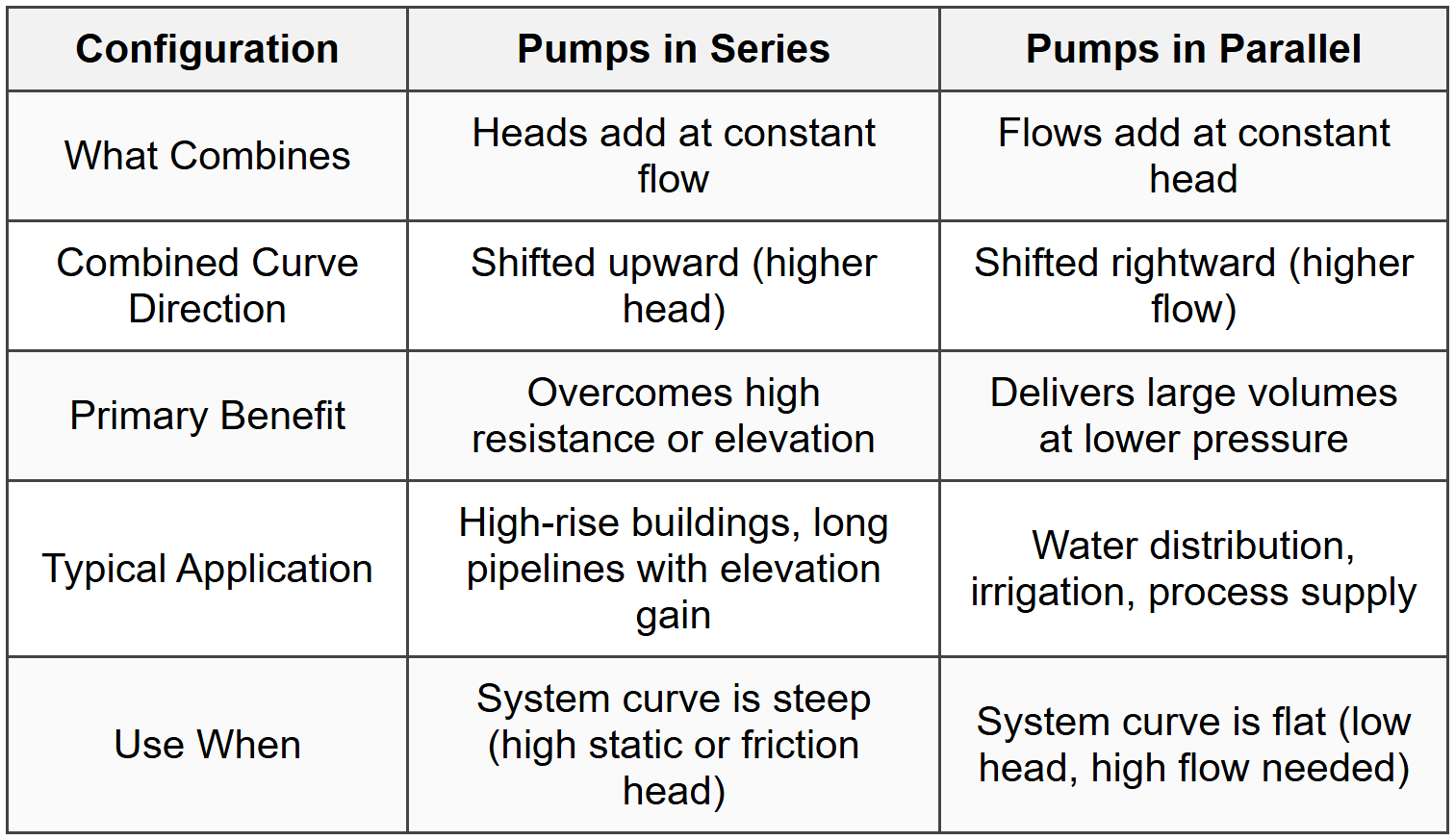
Pumps in Series and Parallel

Pumps in series add their heads together at each flow rate. The combined pump curve is constructed by summing the head values vertically at constant flow. Use series configuration when the system requires high head but not necessarily high flow.

• At any given flow rate: \(H_{\text{total}} = H_1 + H_2\)
• The combined curve is steeper and reaches higher heads
• Best for systems with high static head or long piping with significant friction

Pumps in parallel add their flow rates together at each head. The combined pump curve is constructed by summing the flow values horizontally at constant head. Use parallel configuration when the system requires high flow but not necessarily high head.

• At any given head: \(Q_{\text{total}} = Q_1 + Q_2\)
• The combined curve extends further to the right (higher flow capacity)
• Best for systems with low head requirements but large volume demands
• Each pump shares the load; if one fails, the other can continue operating at reduced capacity

When to Use This

• When the exam specifies multiple pumps and asks for total flow or head
• When selecting between series or parallel configuration to meet system demands
• When analyzing system performance if one pump in a multi-pump setup fails
• When the question asks which configuration increases flow versus which increases pressure

Net Positive Suction Head (NPSH) Considerations

While the pump and system curves determine flow and head, NPSH ensures the pump operates without cavitation. NPSH available (NPSH_A) is the absolute pressure head at the pump inlet minus the vapor pressure head. NPSH required (NPSH_R) is specified by the pump manufacturer and increases with flow rate.

• Safe operation requires NPSH_A ≥ NPSH_R
• Cavitation occurs when NPSH_A < NPSH_R, causing noise, vibration, and damage
• NPSH_A decreases if suction lift increases or fluid temperature rises (higher vapor pressure)
• The operating point must satisfy both the pump/system curve intersection and NPSH requirements

When to Use This

• When the exam asks whether a pump can operate safely at a given suction condition
• When determining the maximum allowable suction lift for a pump
• When diagnosing cavitation problems in a pump system
• When comparing multiple pumps and one has insufficient NPSH margin despite meeting head requirements

Commonly Tested Scenarios / Pitfalls

1. Scenario: The exam provides a pump curve and system curve graph, then asks what happens to flow rate when a valve in the system is partially closed.

Correct Approach: Recognize that closing a valve increases friction head, shifting the system curve upward. The new intersection with the pump curve occurs at a lower flow rate and higher head. Select the answer indicating flow decreases.

Check first: Identify which curve shifts (system curve) and in which direction (upward/steeper).

Do NOT do first: Assume the pump curve changes-the pump itself hasn't changed, only the system resistance.

Why other options are wrong: Options suggesting flow increases misunderstand that added resistance reduces flow; options suggesting head decreases ignore that the pump must work harder against greater friction.

2. Scenario: The exam asks which pump configuration (series or parallel) is best for a system requiring high flow at low pressure.

Correct Approach: Parallel configuration adds flow capacities at the same head, making it ideal for high-volume, low-pressure applications. Choose parallel.

Check first: Determine whether the system needs more flow or more head-this dictates configuration choice.

Do NOT do first: Select series just because two pumps are involved-series adds head, not flow capacity at the same pressure.

Why other options are wrong: Series configuration increases head but doesn't significantly increase flow at low pressures; single larger pump options may not be as flexible or cost-effective.

3. Scenario: The exam presents a pump operating at a point far from its best efficiency point (BEP) and asks about consequences.

Correct Approach: Operating far from BEP increases energy consumption, causes excessive wear, vibration, and heat generation. Select the answer indicating reduced efficiency and potential mechanical problems.

Check first: Confirm where the operating point lies relative to BEP on the pump curve.

Do NOT do first: Assume operation is acceptable as long as the pump delivers the required flow-efficiency and longevity suffer outside BEP.

Why other options are wrong: Options suggesting no impact ignore manufacturer guidelines; options suggesting pump failure is immediate overstate the consequence (it's gradual wear, not instant breakdown).

4. Scenario: The exam asks for the operating flow rate given specific pump and system curve equations or graphs.

Correct Approach: Set the pump head equation equal to the system head equation and solve for flow rate \(Q\), or locate the intersection point on the graph. The intersection defines the operating point.

Check first: Verify units are consistent (gpm vs. cfs, feet vs. meters) before solving or reading the graph.

Do NOT do first: Read the maximum pump capacity or shutoff head as the operating point-these are endpoints, not the actual operating condition.

Why other options are wrong: Maximum flow occurs only with zero head; shutoff head occurs at zero flow; neither represents realistic operation when the system has both static and friction head.

5. Scenario: The exam describes increasing pump speed and asks how the operating point changes.

Correct Approach: Increasing speed shifts the pump curve upward (affinity laws: flow scales with speed, head scales with speed squared). The new operating point moves to higher flow and higher head. Select the answer indicating both increase.

Check first: Identify that pump speed changes affect the pump curve, not the system curve.

Do NOT do first: Assume only flow increases while head stays constant-both parameters change according to affinity laws.

Why other options are wrong: Options suggesting only flow increases ignore the head increase; options suggesting the system curve changes confuse pump modifications with system modifications.

Step-by-Step Procedures or Methods

Task: Determine the operating flow rate and head given pump and system curve equations

1. Write the pump curve equation in the form \(H_{\text{pump}} = f(Q)\), typically a downward-sloping function
2. Write the system curve equation in the form \(H_{\text{system}} = H_{\text{static}} + kQ^2\), where \(H_{\text{static}}\) is constant elevation/pressure head and \(kQ^2\) represents friction losses
3. Set the two equations equal: \(H_{\text{pump}} = H_{\text{system}}\)
4. Solve for \(Q\) (flow rate) using algebra or numerical methods if the equation is nonlinear
5. Substitute \(Q\) back into either equation to find \(H\) (head) at the operating point
6. Verify the solution makes physical sense: positive flow and head, within pump operating range

Task: Graphically determine the operating point from plotted pump and system curves

1. Plot the pump curve with head on the vertical axis and flow rate on the horizontal axis, showing the downward trend
2. Plot the system curve on the same axes, starting at static head when \(Q = 0\) and curving upward
3. Locate the intersection point where the two curves cross
4. Read the flow rate from the horizontal axis at the intersection
5. Read the head from the vertical axis at the intersection
6. Confirm this point satisfies both curves by checking coordinates against curve data

Task: Construct a combined pump curve for two identical pumps in parallel

1. Select a series of head values spanning the operating range
2. For each head value, read the flow rate \(Q_1\) from the single pump curve
3. Since the pumps are identical, the second pump delivers the same \(Q_2 = Q_1\) at that head
4. Calculate total flow: \(Q_{\text{total}} = Q_1 + Q_2 = 2Q_1\)
5. Plot the point \((Q_{\text{total}}, H)\) for each head value
6. Connect the points to form the combined parallel pump curve, which extends further right than the single pump curve

Task: Construct a combined pump curve for two identical pumps in series

1. Select a series of flow rate values spanning the operating range
2. For each flow rate, read the head \(H_1\) from the single pump curve
3. Since the pumps are identical, the second pump adds the same head \(H_2 = H_1\) at that flow
4. Calculate total head: \(H_{\text{total}} = H_1 + H_2 = 2H_1\)
5. Plot the point \((Q, H_{\text{total}})\) for each flow value
6. Connect the points to form the combined series pump curve, which extends higher than the single pump curve

Task: Predict how the operating point changes after a system modification

1. Identify the modification: valve closure, pipe diameter change, elevation change, or pump change
2. Determine which curve is affected: system modifications change the system curve; pump modifications change the pump curve
3. Determine direction of shift: increased resistance shifts system curve up; decreased resistance shifts it down; faster pump shifts pump curve up
4. Sketch or visualize the new curve position
5. Locate the new intersection point with the unchanged curve
6. Compare the new operating point to the original: note whether flow and head increased or decreased

Practice Questions

Q1: A centrifugal pump operates at the intersection of its pump curve and the system curve. If a valve in the discharge line is partially closed, what happens to the operating point?
(a) Flow rate increases, head decreases
(b) Flow rate decreases, head increases
(c) Flow rate increases, head increases
(d) Flow rate decreases, head decreases

Ans: (b)
Partially closing a valve increases system resistance, shifting the system curve upward. The new intersection with the unchanged pump curve occurs at lower flow and higher head because the pump must overcome more resistance. (a) is wrong because added resistance cannot increase flow; (c) is wrong because flow decreases with added resistance; (d) is wrong because head increases, not decreases, when the pump works against greater resistance.

Q2: Two identical pumps are configured in parallel to supply water to a distribution system. Compared to a single pump operating alone, the parallel configuration primarily increases:
(a) Maximum head at zero flow
(b) Flow rate at the same head
(c) Efficiency at all operating points
(d) Net positive suction head available

Ans: (b)
Parallel pumps add their flow rates at the same head, doubling the flow capacity at any given head compared to a single pump. (a) is wrong because parallel configuration does not increase head-that requires series configuration; (c) is wrong because efficiency depends on how close the operating point is to BEP, not the configuration itself; (d) is wrong because NPSH_A depends on suction conditions, not pump arrangement.

Q3: A pump curve is defined by \(H_{\text{pump}} = 100 - 0.01Q^2\) (H in feet, Q in gpm). The system curve is \(H_{\text{system}} = 40 + 0.02Q^2\). What is the operating flow rate?
(a) 20 gpm
(b) 30 gpm
(c) 44.7 gpm
(d) 60 gpm

Ans: (c)
Set equations equal: \(100 - 0.01Q^2 = 40 + 0.02Q^2\)
Rearrange: \(60 = 0.03Q^2\)
Solve: \(Q^2 = 2000\), so \(Q = \sqrt{2000} \approx 44.7\) gpm.
(a), (b), and (d) result from arithmetic errors or incorrect setup-verify by substituting back into both equations to confirm heads match at \(Q = 44.7\) gpm.

Q4: Which of the following system changes would shift the system curve downward and to the right, resulting in increased flow at the new operating point?
(a) Installing a smaller diameter pipe
(b) Increasing the elevation of the discharge point
(c) Replacing a pipe section with a larger diameter pipe
(d) Partially closing a control valve

Ans: (c)
Larger diameter pipe reduces friction losses, shifting the system curve downward (lower head required at each flow rate), which moves the operating point to higher flow. (a) increases friction, shifting the curve upward; (b) increases static head, shifting the curve upward; (d) increases resistance, shifting the curve upward-all decrease flow.

Q5: A pump operates at 1750 rpm and delivers 500 gpm at 80 feet of head. If the speed is increased to 2100 rpm, what is the approximate new head using affinity laws?
(a) 80 feet
(b) 96 feet
(c) 115 feet
(d) 138 feet

Ans: (c)
Head varies with the square of speed ratio: \(H_2 = H_1 \left(\frac{N_2}{N_1}\right)^2 = 80 \left(\frac{2100}{1750}\right)^2 = 80 \times (1.2)^2 = 80 \times 1.44 = 115.2\) feet.
(a) ignores speed change; (b) uses linear speed ratio (wrong-should be squared); (d) incorrectly cubes the speed ratio or uses incorrect affinity law.

Q6: What is the first thing to identify when asked to determine if a pump will cavitate in a given installation?
(a) The best efficiency point on the pump curve
(b) The NPSH available versus NPSH required at the operating point
(c) The shutoff head of the pump
(d) The total dynamic head of the system

Ans: (b)
Cavitation occurs when NPSH_A < NPSH_R, so comparing these values is the first step. (a) relates to efficiency, not cavitation; (c) is irrelevant to suction conditions; (d) addresses discharge head, not suction performance-cavitation depends solely on inlet conditions and NPSH.

Quick Review

• Pump curve slopes downward: higher flow → lower head delivered
• System curve slopes upward: higher flow → higher head required (friction increases with \(Q^2\))
• Operating point is the intersection of pump and system curves-this defines actual flow and head
• Partially closing a valve shifts the system curve upward, decreasing flow and increasing head at the new operating point
• Increasing pipe diameter shifts the system curve downward, increasing flow and decreasing head
• Pumps in series: add heads at constant flow (use for high-head applications)
• Pumps in parallel: add flows at constant head (use for high-volume applications)
• Increasing pump speed shifts the pump curve upward: flow increases linearly with speed, head increases with speed squared
• Operating far from BEP reduces efficiency and increases wear-always prefer operating near BEP
• NPSH_A ≥ NPSH_R is required to prevent cavitation; verify at the operating point flow rate