Chapter Notes: Linear Transformations


Data is everywhere in our world, from test scores to weather measurements to survey responses. Often, we need to transform this data to make it easier to understand, compare, or analyze. A linear transformation is a systematic way of changing every value in a dataset by applying the same mathematical rule. This process preserves the shape of the distribution while shifting or scaling the data. Understanding linear transformations helps us interpret standardized test scores, convert between measurement units, adjust for inflation in economics, and compare datasets that were measured on different scales.
What Is a Linear Transformation?
A linear transformation is a change applied to every data value in a dataset using the same linear equation. The general form is:
\[ Y = a + bX \]In this equation, \( X \) represents the original data value, \( Y \) represents the transformed data value, \( a \) is a constant that shifts the data, and \( b \) is a constant that scales (stretches or compresses) the data. Both \( a \) and \( b \) are fixed numbers that remain the same for every value in the dataset.
The term "linear" comes from the fact that if you graph this relationship, it forms a straight line. Every original value gets mapped to exactly one new value following this rule.
Components of a Linear Transformation
There are two key operations that can occur in a linear transformation:
- Addition or Subtraction (Shifting): The constant \( a \) shifts every value in the dataset by the same amount. Adding a positive number shifts all values up; adding a negative number (or subtracting) shifts all values down.
- Multiplication or Division (Scaling): The constant \( b \) multiplies every value by the same factor. If \( b > 1 \), the data spreads out; if \( 0 < b="">< 1="" \),="" the="" data="" compresses.="" if="" \(="" b="" \)="" is="" negative,="" the="" data="" reflects="" across="" zero="" as="">
These two operations can happen separately or together. Understanding each operation individually helps us predict how the entire dataset will change.
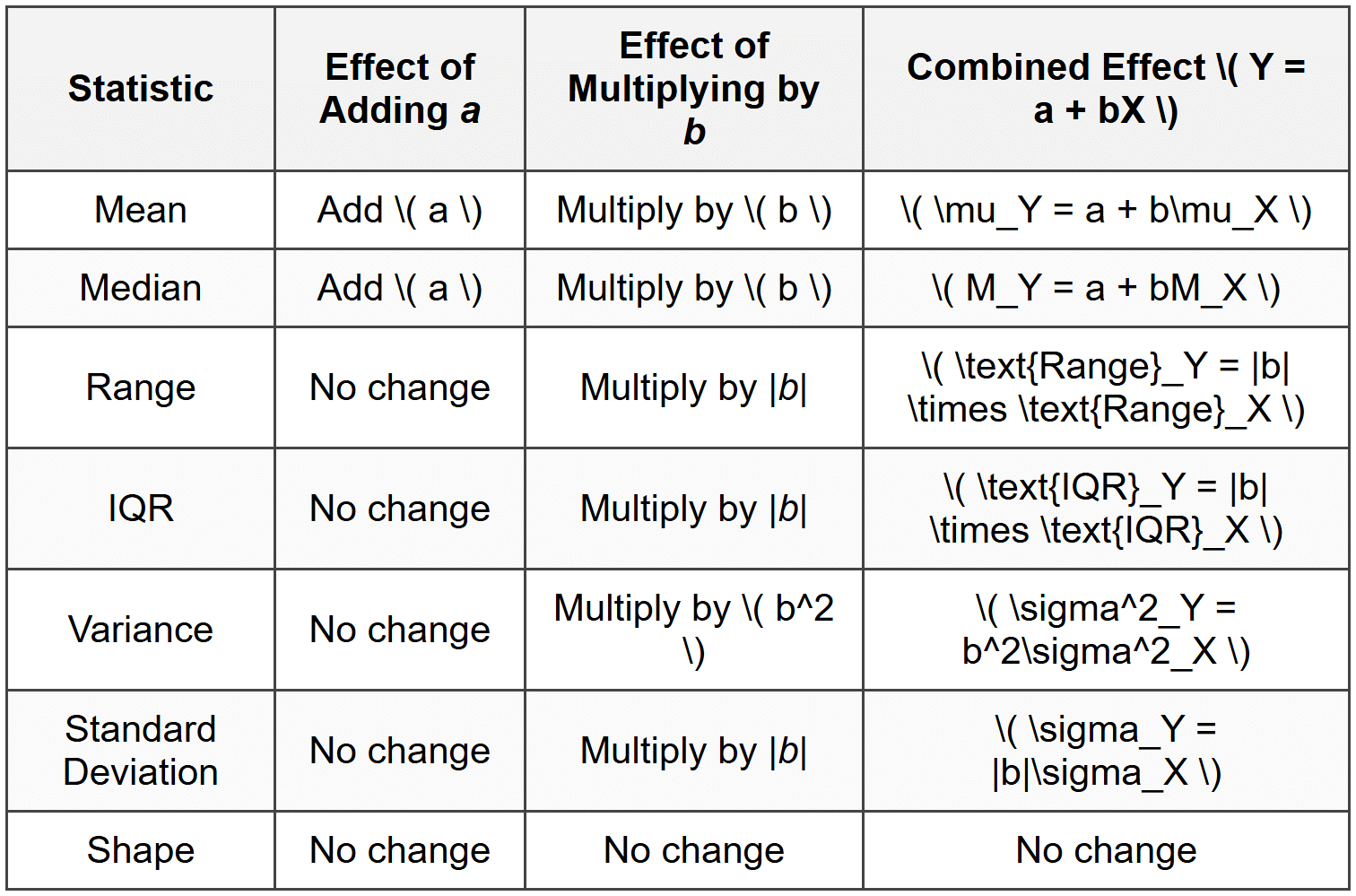
Effects on Measures of Center
When we transform data linearly, the measures of center (mean, median, and mode) transform in predictable ways. This predictability makes linear transformations powerful tools for data analysis.
Transforming the Mean
If every value in a dataset is transformed using \( Y = a + bX \), then the mean of the transformed data follows the same rule:
\[ \text{Mean of } Y = a + b \times (\text{Mean of } X) \]This means the mean transforms exactly like each individual data point. If you add 10 to every test score, the class average increases by exactly 10. If you multiply every measurement by 2, the mean doubles.
Example: A class of students took a quiz, and the mean score was 78 points.
The teacher decides to add 5 bonus points to every student's score.What is the new mean score?
Solution:
The transformation is \( Y = 5 + 1 \times X \), where \( a = 5 \) and \( b = 1 \).
New mean = 5 + 1 × 78
New mean = 5 + 78 = 83 points
The new mean score is 83 points.
Transforming the Median
The median transforms in exactly the same way as the mean:
\[ \text{Median of } Y = a + b \times (\text{Median of } X) \]Since the median is the middle value when data is ordered, shifting all values shifts the middle value by the same amount. Scaling all values scales the middle value proportionally.
Example: The median household income in a town is $52,000.
Due to inflation, all incomes increase by 3%.What is the new median income?
Solution:
A 3% increase means multiplying by 1.03, so the transformation is \( Y = 0 + 1.03 \times X \).
New median = 0 + 1.03 × 52,000
New median = 1.03 × 52,000 = $53,560
The new median household income is $53,560.
Effects on Measures of Spread
Measures of spread describe how data values vary from each other. The most common measures are range, interquartile range (IQR), variance, and standard deviation. Linear transformations affect these measures differently than they affect measures of center.
Adding or Subtracting a Constant
When you add or subtract a constant \( a \) from every data value, measures of spread do not change. This makes intuitive sense: shifting all values by the same amount doesn't make them more or less spread out relative to each other.
- Range stays the same
- IQR stays the same
- Variance stays the same
- Standard deviation stays the same
Think of it like moving a group of people standing in a line. If everyone takes three steps forward together, the distance between any two people doesn't change-they just moved as a group.
Multiplying or Dividing by a Constant
When you multiply every data value by a constant \( b \), measures of spread change according to specific rules:
- Range: Multiplies by the absolute value of \( b \)
- IQR: Multiplies by the absolute value of \( b \)
- Variance: Multiplies by \( b^2 \) (the square of \( b \))
- Standard Deviation: Multiplies by the absolute value of \( b \)
The reason variance multiplies by \( b^2 \) is that variance involves squared deviations from the mean. When each value is multiplied by \( b \), each deviation is multiplied by \( b \), and squaring that gives \( b^2 \).
Example: A dataset of temperatures in Celsius has a mean of 20°C and a standard deviation of 5°C.
Convert these statistics to Fahrenheit using the formula \( F = 32 + 1.8C \).What are the mean and standard deviation in Fahrenheit?
Solution:
Here \( a = 32 \) and \( b = 1.8 \).
Mean in Fahrenheit = 32 + 1.8 × 20 = 32 + 36 = 68°F
Standard deviation in Fahrenheit = |1.8| × 5 = 1.8 × 5 = 9°F
The mean temperature is 68°F with a standard deviation of 9°F. Notice the standard deviation is only affected by the multiplication factor, not by the addition of 32.
Combined Transformations
When both operations occur together (\( Y = a + bX \)):
- The constant \( a \) affects only measures of center (mean, median)
- The constant \( b \) affects both center and spread
- Measures of spread depend only on \( b \), not on \( a \)
Shape of the Distribution
One of the most important properties of linear transformations is that they preserve the shape of a distribution. This means:
- If the original distribution is symmetric, the transformed distribution is symmetric
- If the original distribution is skewed right, the transformed distribution is skewed right
- If the original distribution is skewed left, the transformed distribution is skewed left
- If the original distribution is approximately normal, the transformed distribution is approximately normal
The shape preservation occurs because linear transformations maintain the relative positions of data values. Values that were close together remain close together; values that were far apart remain far apart (proportionally). Outliers remain outliers, though their actual values change.
Imagine a photograph printed on stretchable fabric. You can stretch the fabric horizontally or vertically, and you can shift the entire image left, right, up, or down. The photograph still shows the same scene with the same features in the same relative positions-only the scale and position have changed.
Standardizing Data (Z-Scores)
One of the most important applications of linear transformations in statistics is standardization, also called creating z-scores. This process transforms any dataset to have a mean of 0 and a standard deviation of 1.
The z-score transformation is:
\[ Z = \frac{X - \mu}{\sigma} \]where \( X \) is the original value, \( \mu \) is the mean of the original data, and \( \sigma \) is the standard deviation of the original data. This can be rewritten in the linear transformation form:
\[ Z = -\frac{\mu}{\sigma} + \frac{1}{\sigma} \times X \]Here, \( a = -\frac{\mu}{\sigma} \) and \( b = \frac{1}{\sigma} \).
Purpose of Standardization
Standardizing data serves several important purposes:
- Comparison across different scales: You can compare measurements originally in different units (like test scores and heights)
- Identifying relative position: A z-score tells you how many standard deviations a value is from the mean
- Detecting outliers: Values with z-scores beyond ±2 or ±3 are unusually far from the mean
- Working with normal distributions: Standardized normal distributions can be analyzed using standard tables
Example: On a national exam, the mean score is 500 and the standard deviation is 100.
Sarah scored 650 on this exam.What is Sarah's z-score, and what does it mean?
Solution:
Using the z-score formula with \( X = 650 \), \( \mu = 500 \), and \( \sigma = 100 \):
\( Z = \frac{650 - 500}{100} \)
\( Z = \frac{150}{100} \)
\( Z = 1.5 \)
Sarah's z-score is 1.5, meaning her score is 1.5 standard deviations above the mean.
Interpreting Z-Scores
Z-scores provide a standardized way to describe where a value falls within a distribution:
- A z-score of 0 means the value equals the mean
- A positive z-score means the value is above the mean
- A negative z-score means the value is below the mean
- The magnitude (absolute value) tells how far from the mean in standard deviation units
For approximately normal distributions, about 68% of values have z-scores between -1 and 1, about 95% have z-scores between -2 and 2, and about 99.7% have z-scores between -3 and 3.
Converting Between Units
Many real-world applications of linear transformations involve converting measurements between different unit systems. These conversions are linear transformations because they follow the pattern \( Y = a + bX \).
Common Unit Conversions
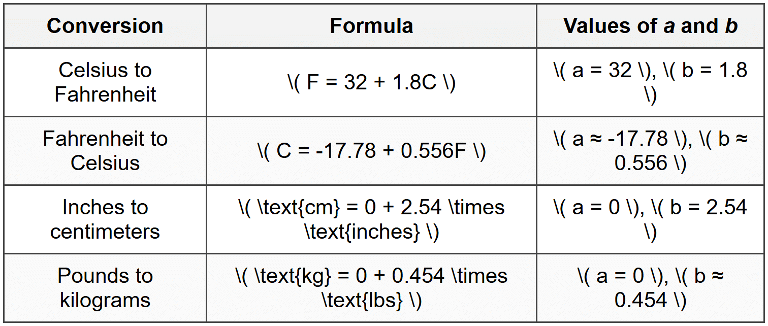
Notice that temperature conversions involve both shifting and scaling (\( a ≠ 0 \) and \( b ≠ 1 \)), while many other unit conversions involve only scaling (\( a = 0 \) and \( b ≠ 1 \)).
Example: A weather station records daily high temperatures in Fahrenheit for a week.
The mean temperature is 77°F with a standard deviation of 6°F.What would these statistics be if converted to Celsius?
Solution:
The conversion formula is \( C = -17.78 + 0.556F \) (approximately).
Mean in Celsius = -17.78 + 0.556 × 77
Mean in Celsius = -17.78 + 42.81 = 25.03°C
Standard deviation in Celsius = |0.556| × 6 = 3.34°C
The mean temperature is approximately 25°C with a standard deviation of approximately 3.3°C.
Summary of Transformation Effects
Understanding how linear transformations affect statistical measures helps you work efficiently with data. Here's a comprehensive summary:
Practical Applications
Linear transformations appear in many real-world contexts beyond simple unit conversions.
Grading and Scoring
Teachers often apply linear transformations to adjust test scores. For example, curving grades by adding points to everyone's score, or converting raw scores to a different scale (like converting to a 100-point scale from a 50-point scale by multiplying by 2).
Economics and Finance
Adjusting for inflation involves applying a linear transformation to historical prices. Converting between currencies is also a linear transformation (when exchange rates are constant).
Scientific Measurement
Scientists routinely convert between measurement systems. Transforming between different pressure units (atmospheres, pascals, PSI), energy units (joules, calories, BTUs), or speed units (meters per second, miles per hour, kilometers per hour) all involve linear transformations.
Data Normalization
In data science and statistics, linear transformations normalize data from different sources to make them comparable. Standardization (z-scores) is the most common approach, but other linear rescaling methods exist, such as min-max scaling that transforms data to fall between 0 and 1.
Example: A researcher measures reaction times in milliseconds.
The dataset has a mean of 245 ms and a standard deviation of 32 ms.
To make the numbers easier to work with, the researcher transforms the data using \( Y = -7.656 + 0.032X \) to create values near 0.What are the mean and standard deviation of the transformed data?
Solution:
Here \( a = -7.656 \) and \( b = 0.032 \).
New mean = -7.656 + 0.032 × 245 = -7.656 + 7.84 = 0.184
New standard deviation = |0.032| × 32 = 1.024
The transformed data has a mean of approximately 0.18 and a standard deviation of approximately 1.02, making the numbers simpler to interpret and analyze.
Inverse Transformations
Every linear transformation has an inverse transformation that reverses the process and returns you to the original values. If the forward transformation is \( Y = a + bX \) (where \( b ≠ 0 \)), the inverse transformation is:
\[ X = -\frac{a}{b} + \frac{1}{b}Y \]This allows you to convert back and forth between scales. For instance, if you convert Celsius to Fahrenheit, you can use the inverse formula to convert Fahrenheit back to Celsius.
Understanding that transformations are reversible is important when interpreting results. If you standardize data, perform an analysis, and need to report results in the original units, you apply the inverse transformation to convert back.
Linear transformations are powerful tools that maintain the essential structure of data while changing the scale or position. By understanding how these transformations affect measures of center, spread, and shape, you gain flexibility in how you analyze, compare, and communicate statistical information across different contexts and measurement systems.
