Chapter Notes: Density Curves

Table of Contents
1. What Is a Density Curve?
2. Finding Areas Under Density Curves
3. Mean and Median of Density Curves
4. Common Density Curves: The Normal Distribution
5. Interpreting and Using Density Curves
6. Working with Combined Areas
7. Practical Applications of Density Curves
View more

When we collect data and create graphs to represent it, we often see patterns emerge. Instead of looking at individual data points, we can sometimes describe the entire distribution with a smooth curve. A density curve is a mathematical model that describes the overall pattern of a distribution. Unlike histograms or dot plots that show actual data, density curves are idealized, smooth representations that help us understand the general shape and behavior of data distributions. Understanding density curves is essential for working with continuous probability distributions and for making inferences about populations based on sample data.

What Is a Density Curve?

A density curve is a curve that is always on or above the horizontal axis and has an area of exactly 1 (or 100%) underneath it. Think of a density curve as a smoothed-out version of a histogram where the bars have been replaced by a continuous line. The curve represents the distribution of a continuous variable, meaning the variable can take on any value within a range rather than just specific, separate values.

Imagine smoothing out a histogram of heights of adult women. Instead of rectangular bars showing how many women fall into each height range, you'd have a smooth curve that flows continuously across all possible heights.

Key Properties of Density Curves

Every density curve must satisfy these essential properties:

• The curve is always on or above the horizontal axis (it never dips below the x-axis)
• The total area under the curve equals exactly 1
• The area under the curve between any two values represents the proportion (or probability) of observations that fall between those values
• The curve describes the overall pattern of the distribution, not individual data points

Because the total area equals 1, we can interpret any portion of that area as a proportion or percentage. For example, if the area under the curve between 60 and 70 equals 0.25, this means that 25% of the observations fall between 60 and 70.

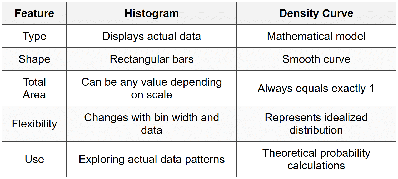
Density Curves vs. Histograms

While histograms display actual data using bars, density curves are mathematical models. Here are the important differences:

Finding Areas Under Density Curves

The fundamental principle of working with density curves is that area represents proportion. When we want to know what fraction of observations fall within a certain range, we calculate the area under the curve between those two values.

Area as Proportion

Since the total area under any density curve equals 1, any portion of that area tells us the proportion of observations in that range. To convert a proportion to a percentage, we multiply by 100.

Example:  A density curve describes test scores on a standardized exam.
The area under the curve between 500 and 600 is 0.34.

What percentage of students scored between 500 and 600?

Solution:

The area under the curve represents the proportion of students who scored in that range.

Proportion = 0.34

Percentage = 0.34 × 100 = 34%

Therefore, 34% of students scored between 500 and 600 on this exam.

Finding Areas for Simple Geometric Shapes

Some density curves have simple geometric shapes like rectangles or triangles. For these curves, we can use basic geometry formulas to calculate areas.

Uniform Density Curves (Rectangular)

A uniform density curve is a horizontal line that creates a rectangle. This represents a uniform distribution where all values in the range are equally likely. The height of the rectangle is determined by the fact that the total area must equal 1.

For a uniform distribution from \( a \) to \( b \), the height is:

where \( a \) is the minimum value and \( b \) is the maximum value.

Example:  A random number generator produces numbers uniformly distributed between 0 and 10.
This means every number between 0 and 10 is equally likely to be selected.

What is the probability that the generator produces a number between 3 and 7?

Solution:

First, find the height of the uniform density curve:

height = 1 ÷ (10 - 0) = 1 ÷ 10 = 0.1

The area of interest is a rectangle with base from 3 to 7:

base = 7 - 3 = 4

Area = base × height = 4 × 0.1 = 0.40

The probability is 0.40 or 40%.

Triangular Density Curves

Some density curves form triangular shapes. To find areas under these curves, we use the triangle area formula:

Example:  A density curve has a triangular shape with its peak at x = 5.
The triangle has a base from x = 0 to x = 10 and a height of 0.2.

What proportion of observations fall between x = 0 and x = 5?

Solution:

The region from x = 0 to x = 5 forms a triangle with:

base = 5 - 0 = 5
height = 0.2

Area = (1/2) × base × height

Area = (1/2) × 5 × 0.2 = (1/2) × 1.0 = 0.5

The proportion of observations between 0 and 5 is 0.5 or 50%.

Mean and Median of Density Curves

Just as we can calculate the mean and median for a dataset, density curves also have measures of center. However, these are based on the mathematical properties of the curve rather than actual data values.

The Median of a Density Curve

The median of a density curve is the point that divides the area under the curve exactly in half. This means the area to the left of the median equals 0.5, and the area to the right of the median also equals 0.5.

Think of the median as the balance point where exactly half the probability (or half the observations) falls on each side.

Example:  A uniform density curve extends from 20 to 40.

What is the median of this distribution?

Solution:

For a uniform distribution, the median is at the midpoint of the range.

Median = (20 + 40) ÷ 2 = 60 ÷ 2 = 30

We can verify: The area from 20 to 30 equals 0.5, and the area from 30 to 40 equals 0.5.

The median is 30.

The Mean of a Density Curve

The mean of a density curve is the balance point of the curve. If you imagine the density curve as a solid shape cut from cardboard, the mean is the point where it would balance perfectly on a knife edge. The mean takes into account not just the location of values but also their density (how much area is concentrated in different regions).

For a symmetric density curve, the mean and median are equal because the distribution is balanced on both sides. For a skewed density curve, the mean is pulled toward the longer tail more than the median.

Mean vs. Median in Skewed Distributions

Understanding the relationship between mean and median helps us understand the shape of a distribution:

• Symmetric distribution: Mean = Median (both are at the center)
• Right-skewed distribution: Mean > Median (the mean is pulled toward the long right tail)
• Left-skewed distribution: Mean < median="" (the="" mean="" is="" pulled="" toward="" the="" long="" left="">

Imagine a classroom where most students score around 80% on a test, but a few students score very low, around 20%. This creates a left-skewed distribution. The mean would be pulled down by those low scores more than the median would be.

Common Density Curves: The Normal Distribution

The most important density curve in statistics is the normal curve, also called the Gaussian curve or bell curve. Many real-world phenomena follow approximately normal distributions: heights, test scores, measurement errors, and many biological and physical measurements.

Properties of Normal Curves

A normal density curve has these distinctive characteristics:

• Bell-shaped and symmetric around its center
• The mean and median are equal and located at the center peak
• The curve extends infinitely in both directions but gets very close to the horizontal axis
• Defined by two parameters: mean (μ) and standard deviation (σ)
• Follows the 68-95-99.7 rule (Empirical Rule)

The 68-95-99.7 Rule

For any normal distribution, we can describe what percentage of observations fall within certain distances from the mean. This is called the Empirical Rule or the 68-95-99.7 Rule:

• Approximately 68% of observations fall within 1 standard deviation of the mean
• Approximately 95% of observations fall within 2 standard deviations of the mean
• Approximately 99.7% of observations fall within 3 standard deviations of the mean

Written with symbols, for a normal distribution with mean μ and standard deviation σ:

• 68% of data falls between μ - σ and μ + σ
• 95% of data falls between μ - 2σ and μ + 2σ
• 99.7% of data falls between μ - 3σ and μ + 3σ

Example:  Adult male heights are approximately normally distributed with a mean of 70 inches and a standard deviation of 3 inches.

Between what two heights do approximately 95% of adult males fall?

Solution:

Using the 68-95-99.7 Rule, 95% of observations fall within 2 standard deviations of the mean.

Mean (μ) = 70 inches
Standard deviation (σ) = 3 inches

Lower boundary = μ - 2σ = 70 - 2(3) = 70 - 6 = 64 inches

Upper boundary = μ + 2σ = 70 + 2(3) = 70 + 6 = 76 inches

Approximately 95% of adult males have heights between 64 inches and 76 inches.

Using the Empirical Rule for More Specific Regions

We can combine parts of the 68-95-99.7 Rule to find proportions in more specific regions. Because the normal curve is symmetric, exactly half of each percentage falls on each side of the mean.

Example:  SAT Math scores are approximately normally distributed with mean 500 and standard deviation 100.

What percentage of students score above 600?

Solution:

First, determine how many standard deviations 600 is from the mean:

600 = 500 + 100 = mean + 1 standard deviation

Using the 68-95-99.7 Rule, 68% of scores fall within 1 standard deviation of the mean (between 400 and 600).

This means 32% of scores fall outside this range (100% - 68% = 32%).

Because the distribution is symmetric, half of this 32% is above 600 and half is below 400.

Percentage above 600 = 32% ÷ 2 = 16%

Approximately 16% of students score above 600 on the SAT Math section.

Interpreting and Using Density Curves

Advantages of Density Curves

Density curves offer several advantages over working directly with data:

• Simplification: A smooth curve is easier to work with mathematically than a large dataset
• Prediction: Once we know the type of distribution, we can make predictions about probabilities
• Standardization: Density curves allow us to compare different distributions on a common scale
• Theoretical foundation: Many statistical inference procedures are based on normal distributions

Limitations of Density Curves

It's important to understand what density curves cannot do:

• They are models, not perfect representations of real data
• Real data may only approximately follow a theoretical distribution
• Outliers or unusual features in actual data may not be captured by a smooth curve
• The appropriateness of a density curve model must be checked before using it

Think of a density curve like a map. A map is useful for navigation and understanding general geography, but it doesn't show every single tree or rock. Similarly, a density curve shows the general pattern but not every individual data point.

Checking if Data Follows a Density Curve Model

Before using a density curve to model data, we should verify that the model is appropriate. Common methods include:

• Creating a histogram or dotplot and comparing its shape to the proposed density curve
• Checking if the percentages predicted by the model match the actual data percentages
• Using a normal probability plot (for checking normality specifically)
• Calculating summary statistics and comparing them to what the model predicts

Working with Combined Areas

Often we need to find probabilities for more complex regions by combining simpler areas. Since probabilities (areas) add together, we can find complex regions by adding or subtracting simpler areas.

Addition Principle

If we have two non-overlapping regions, the total probability is the sum of the individual probabilities:

This works when A and B represent non-overlapping intervals.

Complement Principle

Sometimes it's easier to calculate the probability that something does NOT happen, then subtract from 1. The complement of an event A is "not A," and:

Example:  For a normally distributed variable with mean 50 and standard deviation 10, suppose we want to find the probability that a value is either less than 30 or greater than 70.

What is this probability?

Solution:

First, recognize that 30 and 70 are each 2 standard deviations from the mean:

30 = 50 - 2(10) = mean - 2 standard deviations
70 = 50 + 2(10) = mean + 2 standard deviations

From the 68-95-99.7 Rule, 95% of values fall between 30 and 70.

The remaining 5% fall outside this range (either below 30 or above 70).

Using the complement principle: P(less than 30 or greater than 70) = 1 - 0.95 = 0.05 or 5%

The probability is 5%.

Practical Applications of Density Curves

Density curves are used throughout statistics and in many real-world applications:

• Quality control: Manufacturing processes often produce measurements that follow normal distributions. Density curves help determine acceptable ranges and identify defective products.
• Standardized testing: Test scores are often scaled to follow normal distributions, making it easier to compare scores across different test versions.
• Risk assessment: Insurance companies and financial analysts use density curves to model risks and calculate probabilities of various outcomes.
• Scientific measurement: Measurement errors in scientific instruments often follow normal distributions, helping scientists quantify uncertainty.
• Population studies: Many biological measurements (height, weight, blood pressure) follow approximately normal distributions in large populations.

Understanding density curves provides a foundation for more advanced statistical concepts including confidence intervals, hypothesis testing, and regression analysis. The key principle-that area under the curve represents proportion or probability-connects data analysis to probability theory and enables us to make informed decisions based on patterns in data.