Chapter Notes: Correlation Coefficients


When we study the relationship between two numerical variables, one of the most important questions we can ask is: How strongly are these two variables related? For example, does height predict weight? Does study time correlate with test scores? The correlation coefficient is a single number that measures both the direction and strength of a linear relationship between two quantitative variables. Understanding correlation coefficients allows us to make informed decisions, identify patterns, and assess whether two variables move together in a predictable way.
What Is a Correlation Coefficient?
A correlation coefficient is a numerical value that describes the strength and direction of a linear relationship between two variables. The most commonly used correlation coefficient is the Pearson correlation coefficient, often represented by the symbol \( r \).
The correlation coefficient \( r \) always falls between -1 and +1, inclusive:
- \( r = +1 \): Perfect positive linear relationship. As one variable increases, the other increases in perfect proportion.
- \( r = -1 \): Perfect negative linear relationship. As one variable increases, the other decreases in perfect proportion.
- \( r = 0 \): No linear relationship. Knowing one variable tells us nothing about the other in a linear sense.
- \( 0 < r="">< +1=""> Positive linear relationship. As one variable increases, the other tends to increase, but not perfectly.
- \( -1 < r="">< 0=""> Negative linear relationship. As one variable increases, the other tends to decrease, but not perfectly.
The closer \( |r| \) (the absolute value of \( r \)) is to 1, the stronger the linear relationship. The closer \( r \) is to 0, the weaker the linear relationship.
Think of correlation like a measure of how tightly scattered points cluster around an imaginary straight line. If all the points fall exactly on a line, the correlation is perfect (either +1 or -1). If the points form a cloud with no clear pattern, the correlation is near zero.
Interpreting the Sign and Magnitude of \( r \)
Direction: Positive vs. Negative Correlation
The sign of the correlation coefficient tells us the direction of the relationship:
- Positive correlation (\( r > 0 \)): Both variables tend to increase together. For example, as outdoor temperature increases, ice cream sales tend to increase.
- Negative correlation (\( r < 0=""> As one variable increases, the other tends to decrease. For example, as the amount of time spent exercising increases, resting heart rate tends to decrease.
Strength: How Strong Is the Relationship?
The magnitude (absolute value) of \( r \) tells us how strong the linear relationship is. Here is a common guideline for interpreting the strength of correlation:
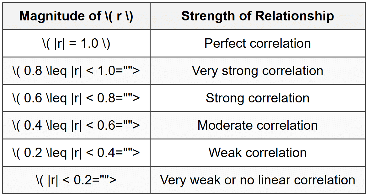
Important: These categories are approximate guidelines. The context of the data matters. In fields like physics, \( r = 0.7 \) might be considered weak, while in social sciences, \( r = 0.5 \) might be considered quite strong.
The Formula for the Pearson Correlation Coefficient
The Pearson correlation coefficient \( r \) can be calculated using the following formula:
\[ r = \frac{\sum (x_i - \bar{x})(y_i - \bar{y})}{\sqrt{\sum (x_i - \bar{x})^2 \sum (y_i - \bar{y})^2}} \]Where:
- \( x_i \) = each individual value of variable \( x \)
- \( y_i \) = each individual value of variable \( y \)
- \( \bar{x} \) = mean (average) of all \( x \) values
- \( \bar{y} \) = mean (average) of all \( y \) values
- \( \sum \) = summation symbol, meaning "add up all the values"
This formula measures how the deviations of \( x \) and \( y \) from their respective means move together, standardized by the variability in each variable.
Alternative Computational Formula
A computational version of the formula that is sometimes easier to use with raw data is:
\[ r = \frac{n \sum x_i y_i - (\sum x_i)(\sum y_i)}{\sqrt{[n \sum x_i^2 - (\sum x_i)^2][n \sum y_i^2 - (\sum y_i)^2]}} \]Where:
- \( n \) = number of data pairs
- \( \sum x_i y_i \) = sum of the products of paired \( x \) and \( y \) values
- \( \sum x_i \) = sum of all \( x \) values
- \( \sum y_i \) = sum of all \( y \) values
- \( \sum x_i^2 \) = sum of the squares of all \( x \) values
- \( \sum y_i^2 \) = sum of the squares of all \( y \) values
In practice, most statisticians use technology (graphing calculators, Excel, statistical software) to compute \( r \), but understanding the formula helps you appreciate what the correlation coefficient measures.
Calculating the Correlation Coefficient: Step-by-Step Example
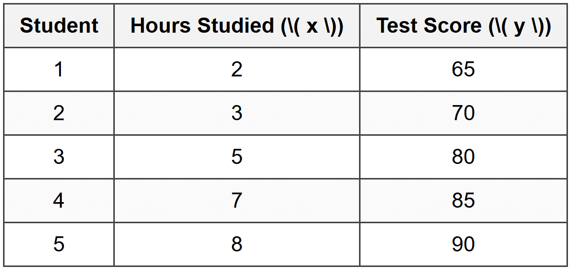
Example: A teacher wants to study the relationship between hours studied and test scores.
Five students provided the following data:Calculate the Pearson correlation coefficient \( r \).
Solution:
Step 1: Calculate the means of \( x \) and \( y \).
\( \bar{x} = \frac{2 + 3 + 5 + 7 + 8}{5} = \frac{25}{5} = 5 \)
\( \bar{y} = \frac{65 + 70 + 80 + 85 + 90}{5} = \frac{390}{5} = 78 \)
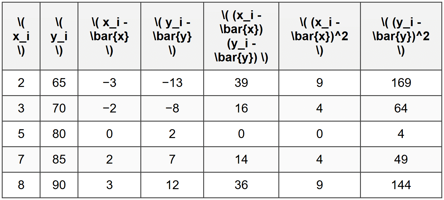
Step 2: Compute the deviations from the mean for each data point, and their products and squares.
Step 3: Sum the columns.
\( \sum (x_i - \bar{x})(y_i - \bar{y}) = 39 + 16 + 0 + 14 + 36 = 105 \)
\( \sum (x_i - \bar{x})^2 = 9 + 4 + 0 + 4 + 9 = 26 \)
\( \sum (y_i - \bar{y})^2 = 169 + 64 + 4 + 49 + 144 = 430 \)
Step 4: Plug the values into the correlation formula.
\[ r = \frac{105}{\sqrt{26 \times 430}} = \frac{105}{\sqrt{11180}} = \frac{105}{105.73} \approx 0.993 \]The correlation coefficient is approximately 0.993.
This indicates a very strong positive linear relationship between hours studied and test scores.
Properties of the Correlation Coefficient
Understanding the properties of \( r \) helps you interpret correlation correctly and avoid common mistakes.
Property 1: Correlation Is Unitless
The correlation coefficient \( r \) has no units. Whether you measure height in inches or centimeters, or weight in pounds or kilograms, the value of \( r \) remains the same. This makes correlation a universal measure of association.
Property 2: Correlation Measures Only Linear Relationships
Correlation detects linear patterns-relationships that can be approximated by a straight line. If two variables have a strong curved (nonlinear) relationship, \( r \) may be close to zero even though the variables are closely related.
For example, the relationship between the height of a ball thrown upward and time is quadratic (a parabola). Even though the variables are perfectly related, the Pearson correlation coefficient will not be +1 or -1 because the relationship is not linear.
Property 3: Correlation Does Not Imply Causation
This is one of the most critical principles in statistics. A high correlation between two variables does not mean that one causes the other. Both variables might be influenced by a third lurking variable, or the association might be coincidental.
For example, ice cream sales and drowning incidents are positively correlated. This does not mean eating ice cream causes drowning. Instead, both increase during hot summer months-a lurking variable.
Property 4: Outliers Can Strongly Affect Correlation
Because the formula for \( r \) involves squaring deviations, a single extreme data point (outlier) can have a large effect on the correlation coefficient. It's important to inspect scatterplots and check for outliers before interpreting \( r \).
Property 5: Switching \( x \) and \( y \) Does Not Change \( r \)
The correlation between \( x \) and \( y \) is the same as the correlation between \( y \) and \( x \). This symmetry reflects the fact that correlation measures association, not causation or prediction direction.
Using Scatterplots to Visualize Correlation
A scatterplot is a graph that displays paired numerical data as individual points. The horizontal axis represents one variable, and the vertical axis represents the other. Scatterplots are the primary visual tool for assessing correlation.
What to Look For in a Scatterplot
- Direction: Do the points trend upward (positive) or downward (negative)?
- Form: Do the points cluster around a straight line (linear) or follow a curve (nonlinear)?
- Strength: How tightly do the points cluster around the pattern? Tight clustering means strong correlation; loose scatter means weak correlation.
- Outliers: Are there any points that do not fit the general pattern?
Always create and examine a scatterplot before calculating or interpreting a correlation coefficient. The scatterplot reveals the full story of the relationship, while \( r \) is just a single summary number.
Examples of Different Correlation Strengths
Example: Interpret the following correlation coefficients in context.
(a) \( r = 0.92 \) between hours of sleep and test performance.
Solution:
This indicates a very strong positive correlation.
As hours of sleep increase, test performance tends to increase substantially.
The relationship is strong and positive, meaning more sleep is strongly associated with better test performance.
Example: (b) \( r = -0.65 \) between screen time before bed and sleep quality.
Solution:
This indicates a strong negative correlation.
As screen time before bed increases, sleep quality tends to decrease.
The negative sign shows the inverse relationship, meaning more screen time is strongly associated with poorer sleep quality.
Example: (c) \( r = 0.15 \) between shoe size and GPA among high school students.
Solution:
This indicates a very weak or negligible positive correlation.
Knowing a student's shoe size tells us almost nothing about their GPA.
The correlation is so weak that the relationship is effectively nonexistent.
Coefficient of Determination: \( r^2 \)
While the correlation coefficient \( r \) measures the strength and direction of a linear relationship, the coefficient of determination, denoted \( r^2 \), tells us the proportion of variation in one variable that can be explained by the other variable.
If \( r = 0.8 \), then:
\[ r^2 = (0.8)^2 = 0.64 \]This means that 64% of the variation in the dependent variable can be explained by the independent variable through the linear relationship. The remaining 36% is due to other factors or randomness.
Interpreting \( r^2 \)
- \( r^2 = 0 \): The independent variable explains none of the variation in the dependent variable.
- \( r^2 = 1 \): The independent variable explains all of the variation in the dependent variable.
- \( r^2 \) is always between 0 and 1, regardless of whether \( r \) is positive or negative.
Example: If the correlation between study time and test scores is \( r = 0.9 \), what percentage of the variation in test scores is explained by study time?
Solution:
\( r^2 = (0.9)^2 = 0.81 \)
This means 81% of the variation in test scores can be explained by differences in study time.
The remaining 19% is due to other factors, such as prior knowledge, test anxiety, or sleep.
Common Misinterpretations and Cautions
Mistaking Correlation for Causation
Just because two variables are correlated does not mean one causes the other. Establishing causation requires controlled experiments, not just observational correlation.
Ignoring Nonlinear Relationships
A correlation coefficient near zero does not mean there is no relationship-it means there is no linear relationship. Always check the scatterplot to see if a curved pattern exists.
Extrapolating Beyond the Data
Correlation describes the relationship within the range of observed data. Extending conclusions beyond that range (extrapolation) can lead to incorrect predictions.
Assuming Correlation Applies to Individuals
Correlation describes group trends. A positive correlation between study time and test scores does not guarantee that every individual who studies more will score higher.
Using Technology to Calculate Correlation
In practice, correlation coefficients are almost always computed using technology:
- Graphing calculators: Most have built-in functions to compute \( r \) from lists of data.
- Spreadsheet software (Excel, Google Sheets): Use the function
=CORREL(array1, array2). - Statistical software (R, Python, SPSS): Dedicated correlation functions provide \( r \), \( r^2 \), and significance tests.
While technology handles the computation, understanding what \( r \) measures and how to interpret it remains essential.
Summary of Key Ideas
- The correlation coefficient \( r \) measures the strength and direction of a linear relationship between two quantitative variables.
- \( r \) ranges from -1 to +1. Values near +1 indicate strong positive correlation; values near -1 indicate strong negative correlation; values near 0 indicate weak or no linear correlation.
- Correlation is unitless and does not change if you switch \( x \) and \( y \).
- Correlation measures only linear relationships. Nonlinear patterns may not be detected by \( r \).
- Correlation does not imply causation. Association does not prove that one variable causes changes in the other.
- The coefficient of determination \( r^2 \) indicates the proportion of variation in one variable explained by the other.
- Always create and examine a scatterplot before interpreting \( r \).
- Outliers can strongly influence the value of \( r \).
Mastering correlation coefficients equips you with a powerful tool for exploring relationships in data, making informed predictions, and thinking critically about statistical claims you encounter in science, news, and everyday life.


