Chapter Notes: Assessing The Fit in Least-Squares Regression


When we create a least-squares regression line to model the relationship between two quantitative variables, we're making predictions based on a pattern in the data. But how well does that line actually fit the data? Does it capture most of the variability, or does it miss important patterns? Assessing the fit means evaluating how closely the regression line matches the actual data points and whether the line is appropriate for making predictions. In this chapter, we'll learn several methods to determine whether our linear model is doing a good job, including examining residuals, calculating the coefficient of determination, and checking key conditions that must be met for the model to be valid.
Understanding Residuals
A residual is the difference between an observed data value and the value predicted by the regression line. In plain English, it tells us how far off our prediction was. If we have an actual \( y \)-value and our regression line predicts \( \hat{y} \) (read as "y-hat"), then the residual is calculated as:
\[ \text{residual} = y - \hat{y} \]where \( y \) is the observed value and \( \hat{y} \) is the predicted value from the regression equation.
A positive residual means the actual data point is above the regression line-our model underestimated the value. A negative residual means the actual data point is below the regression line-our model overestimated the value. A residual of zero means the point lies exactly on the line, which is rare with real data.
Think of residuals as the "leftover" distances after the regression line has done its best to fit the data. If you were throwing darts at a target, residuals would measure how far each dart landed from the bullseye.
Calculating Residuals
To calculate residuals, we follow these steps for each data point:
- Use the regression equation to calculate the predicted value \( \hat{y} \) by plugging in the \( x \)-value.
- Subtract the predicted value from the actual \( y \)-value.
- Record whether the residual is positive, negative, or zero.
Example: A researcher studying the relationship between hours of study and test scores finds the regression equation \( \hat{y} = 50 + 5x \), where \( x \) is hours studied and \( y \) is the test score.
One student studied 6 hours and scored 82 on the test.What is the residual for this student?
Solution:
First, we calculate the predicted score using the regression equation:
\( \hat{y} = 50 + 5(6) = 50 + 30 = 80 \)
Next, we calculate the residual:
residual = \( y - \hat{y} = 82 - 80 = 2 \)
The residual is 2 points, meaning the student scored 2 points higher than the model predicted.
The Sum and Mean of Residuals
An important mathematical property of least-squares regression is that the sum of all residuals always equals zero (or very close to zero, accounting for rounding). This happens because the regression line is positioned to balance the positive and negative deviations. Because of this property, we cannot use the sum of residuals to assess fit-it will always be zero regardless of how well the line fits.
Instead, we examine residuals in other ways, particularly through residual plots and by calculating the standard deviation of residuals.
Residual Plots
A residual plot is a scatterplot that displays the residuals on the vertical axis and either the explanatory variable \( x \) or the predicted values \( \hat{y} \) on the horizontal axis. Residual plots are powerful diagnostic tools because they help us see patterns that indicate whether a linear model is appropriate.
Interpreting Residual Plots
When a linear model is appropriate and the conditions for regression are met, the residual plot should show:
- Random scatter with no clear pattern
- Points roughly evenly distributed above and below the horizontal line at residual = 0
- Approximately constant vertical spread (variability) across all \( x \)-values
If the residual plot shows a curved pattern, this suggests that the relationship between the variables is not linear, and a linear model is not appropriate. For example, if the residuals form a U-shape or an upside-down U-shape, the relationship may be quadratic or exponential.
If the residual plot shows a fan shape or funnel shape, where the spread of residuals increases or decreases as \( x \) increases, this indicates that the variability in \( y \) is not constant. This violates the condition of constant variance and suggests the model may not be reliable for all \( x \)-values.
A good residual plot looks like a random cloud of points centered around zero, like stars scattered randomly in the night sky. A bad residual plot shows a clear pattern or shape, like a smiley face or a megaphone.
What to Look For in Residual Plots
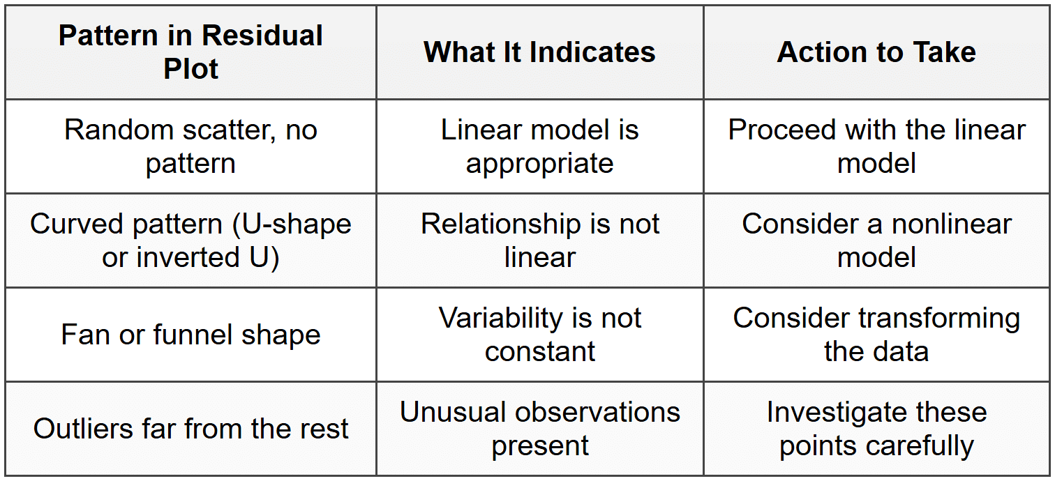
Standard Deviation of Residuals
The standard deviation of residuals, often denoted \( s \) or \( s_e \), measures the typical distance that observed values fall from the regression line. It quantifies the average size of the prediction errors and is calculated using the formula:
\[ s = \sqrt{\frac{\sum (y - \hat{y})^2}{n - 2}} \]where the numerator is the sum of squared residuals, and \( n - 2 \) is the degrees of freedom (we subtract 2 because we estimated two parameters: the slope and intercept).
A smaller value of \( s \) indicates that the data points cluster more tightly around the regression line, meaning the model makes more accurate predictions. A larger value of \( s \) indicates greater scatter and less precise predictions.
Think of the standard deviation of residuals as a measure of prediction accuracy. If \( s = 5 \) points on a test score regression, it means our predictions are typically off by about 5 points in either direction.
The value of \( s \) is reported in the same units as the response variable \( y \), which makes it easy to interpret in context. For example, if we're predicting home prices in dollars and \( s = 15,000 \), our typical prediction error is about $15,000.
Example: A regression model predicting fuel efficiency (in miles per gallon) from vehicle weight has a standard deviation of residuals \( s = 3.2 \) mpg.
What does this value tell us about the model's predictions?
Solution:
The standard deviation of residuals is 3.2 mpg.
This means that the actual fuel efficiency values typically differ from the predicted values by about 3.2 miles per gallon.
In other words, when we use this model to predict a car's fuel efficiency, our prediction will typically be off by roughly 3.2 mpg in either direction.
Coefficient of Determination (r²)
The coefficient of determination, denoted \( r^2 \) (read as "r-squared"), measures the proportion of variability in the response variable \( y \) that is explained by the least-squares regression line using the explanatory variable \( x \). It is calculated by squaring the correlation coefficient \( r \).
The value of \( r^2 \) always falls between 0 and 1 (or between 0% and 100% when expressed as a percentage):
- \( r^2 = 0 \) means the regression line explains none of the variability in \( y \)-the line provides no useful predictions.
- \( r^2 = 1 \) means the regression line explains all of the variability in \( y \)-every data point falls exactly on the line.
- Values between 0 and 1 indicate partial explanation of the variability.
Interpreting r²
When we interpret \( r^2 \), we always express it as a percentage and use this template:
"About [value]% of the variation in [response variable] is accounted for by the linear model relating [response variable] to [explanatory variable]."
For example, if \( r^2 = 0.64 \) in a model predicting test scores from hours studied, we would say: "About 64% of the variation in test scores is accounted for by the linear model relating test scores to hours studied."
The remaining 36% of the variation is due to other factors not included in the model, such as prior knowledge, test anxiety, sleep quality, or random chance.
Example: A study examining the relationship between daily exercise time (in minutes) and resting heart rate (in beats per minute) produces a correlation of \( r = -0.75 \).
Calculate and interpret \( r^2 \).
Solution:
We calculate \( r^2 \) by squaring the correlation coefficient:
\( r^2 = (-0.75)^2 = 0.5625 \)
Converting to a percentage: \( 0.5625 × 100 = 56.25\% \)
Interpretation: About 56.25% of the variation in resting heart rate is accounted for by the linear model relating resting heart rate to daily exercise time.
What r² Does NOT Tell Us
It's important to understand what \( r^2 \) does not indicate:
- \( r^2 \) does not tell us whether the relationship is linear-we need a residual plot for that.
- \( r^2 \) does not tell us the slope of the line or the strength of the relationship in the original units.
- \( r^2 \) does not prove causation-a high \( r^2 \) can occur even when there is no causal relationship.
- \( r^2 \) does not indicate whether the model is appropriate for prediction-even with high \( r^2 \), we must check conditions.
Conditions for Regression
For the least-squares regression model to be valid and our predictions trustworthy, four key conditions must be met. These conditions ensure that the mathematical assumptions underlying regression inference are satisfied.
1. Linearity
The relationship between the explanatory variable \( x \) and the response variable \( y \) must be approximately linear. We check this condition by:
- Examining the scatterplot of \( y \) versus \( x \) to see if the points follow a roughly straight-line pattern
- Looking at the residual plot to confirm there is no curved pattern
If the linearity condition is violated, a linear model will produce biased predictions and should not be used. Consider transforming the data or using a nonlinear model instead.
2. Independence
The observations must be independent of one another. This means that knowing the value of one observation should not give us information about another observation. We check this condition by considering:
- How the data were collected-was it a random sample or randomized experiment?
- Whether observations are related over time or space
- The study design and context
Common violations include measuring the same subjects multiple times, collecting data over time where consecutive observations are related, or sampling individuals from the same family or location.
3. Constant Variance (Equal Spread)
The variability of the residuals should be approximately constant across all values of \( x \). This condition is also called homoscedasticity. We check this by examining the residual plot:
- The vertical spread of points should be roughly the same across the entire plot
- There should be no fan or funnel shape
- The scatter around zero should not increase or decrease systematically
If variance is not constant, predictions will be more reliable for some \( x \)-values than others, and inference procedures may give incorrect results.
4. Normality of Residuals
The residuals should follow an approximately normal distribution. This condition becomes more important when we're doing inference (confidence intervals and hypothesis tests) rather than just fitting a line. We check this condition by:
- Creating a histogram or dotplot of the residuals to see if the distribution is roughly symmetric and bell-shaped
- Making a normal probability plot (also called a Q-Q plot) of the residuals-if the points follow a roughly straight line, the normality condition is satisfied
Minor departures from normality are acceptable, especially with larger sample sizes. Severe skewness or outliers may require transformation of the data.
Remember the acronym LINE to check regression conditions: Linearity, Independence, Normality, and Equal variance.
Outliers and Influential Points
Individual observations can have varying degrees of influence on the regression line. Understanding which points have unusual influence helps us assess whether our model is driven by the overall pattern or by just a few unusual cases.
Outliers in Regression
An outlier in regression is an observation that has a large residual-it falls far from the regression line. Outliers can be identified in the residual plot as points that are unusually far above or below zero. We can also identify them by calculating standardized residuals and flagging any observations with values beyond ±2 or ±3.
However, not all outliers are problematic. An outlier that falls in line with the \( x \)-values of the rest of the data may have little impact on the slope or intercept.
Influential Points
An influential point is an observation that, if removed, would substantially change the regression line (particularly the slope). Influential points typically have:
- An extreme \( x \)-value (far from the mean of \( x \))
- A \( y \)-value that does not follow the pattern of the other points
A point can be influential without being an outlier in the \( y \)-direction if it has sufficient leverage due to an extreme \( x \)-value.
Think of influential points as having a long lever arm. Just as it's easier to move a heavy door when you push far from the hinge, a point far from the mean \( x \)-value can "pull" the regression line toward itself.
What to Do About Unusual Points
When you identify outliers or influential points, follow these steps:
- Investigate the point-check for data entry errors, measurement problems, or special circumstances
- Consider context-determine whether the point represents valid data or an error
- Analyze with and without-fit the regression both including and excluding the point to see its impact
- Report transparently-document any points removed and justify the decision
Never remove data points simply to improve \( r^2 \) or make the model look better. Only remove points when there is clear justification, such as measurement error or the point representing a different population.
Putting It All Together: Assessing Model Quality
To fully assess whether a regression model fits the data well and is appropriate for making predictions, we combine multiple approaches:
- Create and examine a residual plot to check for linearity and constant variance
- Calculate and interpret \( r^2 \) to understand how much variation the model explains
- Calculate and interpret \( s \) to understand the typical prediction error
- Check all regression conditions (LINE) systematically
- Identify and investigate any outliers or influential points
- Consider the context-does the model make practical sense?
A model with high \( r^2 \) and small \( s \) is not necessarily a good model if the conditions are violated or if the residual plot shows concerning patterns. Conversely, a model with moderate \( r^2 \) can still be useful if the conditions are met and the predictions are meaningful in context.
Example: A researcher models the relationship between advertising spending (in thousands of dollars) and monthly sales (in thousands of dollars) for 30 retail stores.
The regression equation is \( \hat{y} = 120 + 3.5x \).
The correlation is \( r = 0.82 \) and the standard deviation of residuals is \( s = 8.3 \).
The residual plot shows random scatter with no pattern.Assess the quality of this regression model.
Solution:
First, calculate \( r^2 \): \( r^2 = (0.82)^2 = 0.6724 \) or about 67.24%
Interpretation of \( r^2 \): About 67% of the variation in monthly sales is explained by the linear model relating sales to advertising spending. This indicates a reasonably strong relationship.
Interpretation of \( s \): The typical prediction error is about $8,300 (since the units are thousands of dollars). When predicting monthly sales, our predictions are typically off by this amount.
Assessment of conditions: The residual plot shows random scatter with no pattern, suggesting the linearity and constant variance conditions are met. Assuming the stores were selected independently and residuals are approximately normal, all conditions appear satisfied.
Overall assessment: This model provides a reasonably good fit. It explains about two-thirds of the variation in sales, has acceptable prediction accuracy for business planning, and meets the necessary conditions for valid inference.
By systematically assessing the fit of a least-squares regression model, we ensure that our predictions are reliable, our interpretations are valid, and our conclusions are supported by appropriate statistical methods. Always remember that statistical significance or high \( r^2 \) alone does not guarantee a useful or appropriate model-careful checking of conditions and examination of residuals are essential parts of responsible data analysis.


