Chapter Notes: Discrete Random Variables


In probability and statistics, we often work with experiments or processes that produce numerical outcomes. When we roll a die, the result is a number. When we count the number of heads in three coin flips, we get a number. When we survey students to see how many pets they own, we collect numbers. A discrete random variable is a mathematical tool that helps us organize, describe, and analyze these numerical outcomes in a systematic way. Understanding discrete random variables allows us to calculate probabilities, predict outcomes, and make informed decisions based on data.
What Is a Random Variable?
A random variable is a function that assigns a numerical value to each outcome of a random experiment. In plain English, it's a way of turning the results of an experiment into numbers we can work with mathematically.
Let's think about this using a simple example. Suppose you flip a coin three times and you want to know how many heads appear. The possible outcomes of three coin flips might be HHH, HHT, HTH, HTT, THH, THT, TTH, or TTT. Instead of working with these letter combinations, we can define a random variable \( X \) that represents the number of heads. Then:
- If the outcome is HHH, then \( X = 3 \)
- If the outcome is HHT, HTH, or THH, then \( X = 2 \)
- If the outcome is HTT, THT, or TTH, then \( X = 1 \)
- If the outcome is TTT, then \( X = 0 \)
Notice that \( X \) takes the outcomes of the experiment (combinations of heads and tails) and converts them into numbers (0, 1, 2, or 3). This numerical representation makes it much easier to calculate probabilities and perform statistical analysis.
We typically use capital letters like \( X \), \( Y \), or \( Z \) to represent random variables. Once the experiment is performed and we observe a specific value, we use lowercase letters like \( x \), \( y \), or \( z \) to represent that particular outcome.
Discrete vs. Continuous Random Variables
Random variables come in two main types: discrete and continuous. The distinction between them is important for determining which statistical methods to use.
A discrete random variable can only take on specific, separate values. You can list all possible values, even if the list is very long or infinite. These values are often (but not always) whole numbers. Common examples include:
- The number of students absent from class (0, 1, 2, 3, ...)
- The result of rolling a six-sided die (1, 2, 3, 4, 5, 6)
- The number of cars passing through an intersection in one hour (0, 1, 2, 3, ...)
- The number of correct answers on a 10-question quiz (0, 1, 2, ..., 10)
A continuous random variable, by contrast, can take on any value within an interval or range. The possible values cannot be listed individually because there are infinitely many values even in a small range. Examples include:
- The exact height of a randomly selected student (could be 165.2 cm, 165.23 cm, 165.234 cm, etc.)
- The time it takes to run a race (could be any positive number of seconds)
- The temperature at noon (could be any value on a continuous scale)
This chapter focuses exclusively on discrete random variables. The key characteristic to remember is that discrete random variables have countable possible values with gaps between them.
Probability Distribution of a Discrete Random Variable
Once we define a discrete random variable, we need a way to describe the likelihood of each possible value occurring. The probability distribution of a discrete random variable is a complete listing of all possible values the variable can take, along with the probability of each value.
For a discrete random variable \( X \), we write \( P(X = x) \) to mean "the probability that the random variable \( X \) takes on the specific value \( x \)." This is sometimes shortened to \( P(x) \) when the context is clear.
Requirements for a Valid Probability Distribution
Not just any set of numbers can be a probability distribution. For a list of probabilities to be valid, two conditions must be satisfied:
- Each probability must be between 0 and 1 (inclusive): For every possible value \( x \), we must have \( 0 \leq P(X = x) \leq 1 \). Probabilities cannot be negative, and they cannot exceed 1.
- The probabilities must sum to 1: When you add up the probabilities for all possible values, the total must equal exactly 1. Mathematically, \( \sum P(X = x) = 1 \), where the sum is taken over all possible values of \( X \).
These two rules ensure that our probability distribution is logically consistent and represents a complete picture of all possible outcomes.
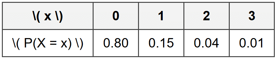
Example: A quality control inspector examines smartphones coming off an assembly line.
Each phone is checked for defects, and the inspector records the number of defects found.
Based on historical data, the probability distribution for \( X \) (the number of defects per phone) is:Verify that this is a valid probability distribution.
Solution:
First, check that each probability is between 0 and 1:
All values (0.80, 0.15, 0.04, 0.01) are between 0 and 1. ✓
Second, check that the probabilities sum to 1:
0.80 + 0.15 + 0.04 + 0.01 = 1.00 ✓
Both conditions are satisfied, so this is a valid probability distribution.
Representing Probability Distributions
There are three common ways to represent the probability distribution of a discrete random variable:
- Table: A two-row or two-column table showing each value and its probability (as shown in the example above)
- Formula: A mathematical function that gives \( P(X = x) \) for any value \( x \)
- Graph: A visual representation, typically a histogram or bar chart, where the height of each bar represents the probability
Each representation has advantages. Tables are easy to read for small numbers of values. Formulas are compact and useful for calculations. Graphs provide visual insight into the shape and spread of the distribution.
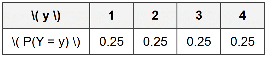
Example: A carnival game involves spinning a wheel divided into four equal sections numbered 1, 2, 3, and 4.
Let \( Y \) represent the number that comes up on a single spin.
Create the probability distribution table for \( Y \).What is the probability distribution?
Solution:
Since the wheel has four equal sections, each number has an equal chance of appearing.
The probability for each outcome is \( \frac{1}{4} = 0.25 \).
The probability distribution table is:
The probability of landing on any particular number is 0.25 or 25%.
Expected Value (Mean) of a Discrete Random Variable
One of the most important characteristics of a probability distribution is its center. The expected value, also called the mean of a discrete random variable, tells us the long-run average value we would expect if we repeated the random experiment many, many times.
The expected value is denoted by \( E(X) \) or by the Greek letter \( \mu \) (mu). Despite its name, the expected value is not necessarily a value we "expect" to see on any single trial. Rather, it represents the theoretical average over many trials.
To calculate the expected value of a discrete random variable \( X \), we use this formula:
\[ E(X) = \mu = \sum x \cdot P(X = x) \]In words: multiply each possible value by its probability, then add up all these products. The symbol \( \sum \) means "sum over all possible values of \( x \)."
Example: An insurance company analyzes claims for a particular type of policy.
Let \( X \) represent the claim amount (in thousands of dollars) with the following distribution:Find the expected claim amount.
Solution:
Use the formula \( E(X) = \sum x \cdot P(X = x) \):
\( E(X) = (0)(0.85) + (1)(0.10) + (5)(0.04) + (10)(0.01) \)
\( E(X) = 0 + 0.10 + 0.20 + 0.10 \)
\( E(X) = 0.40 \)
The expected claim amount is $400 (since \( X \) was measured in thousands of dollars).
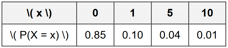
Notice in this example that the expected value is 0.40 (or $400), which is not even one of the possible claim amounts. This illustrates that the expected value represents a long-run average, not a value that will necessarily occur on any single claim.
Interpreting Expected Value
Think of expected value like this: if the insurance company processes thousands of these policies, the average claim amount will approach $400 per policy. Some policies will have no claim, some will have small claims, and a few will have large claims. But averaged over many policies, the company expects to pay out about $400 per policy.
Expected value is extremely useful for making decisions. Companies use it to set prices, determine whether a business venture is profitable, and manage risk. Individuals use it (often without realizing it) when deciding whether to buy insurance, play a game, or make an investment.
Variance and Standard Deviation
While the expected value tells us the center of a distribution, it doesn't tell us anything about how spread out the values are. Two random variables could have the same expected value but very different distributions-one might have values clustered tightly around the mean, while another might have values spread far apart.
The variance measures how much the values of a random variable tend to vary from the expected value. It gives us a numerical measure of spread or dispersion. The variance is denoted by \( \text{Var}(X) \) or \( \sigma^2 \) (sigma squared).
The formula for the variance of a discrete random variable is:
\[ \text{Var}(X) = \sigma^2 = \sum (x - \mu)^2 \cdot P(X = x) \]This formula says: for each possible value \( x \), find how far it is from the mean \( \mu \), square that distance, multiply by the probability, then sum up all these products.
There's an alternative formula that's often easier for calculations:
\[ \text{Var}(X) = E(X^2) - [E(X)]^2 \]where \( E(X^2) = \sum x^2 \cdot P(X = x) \). This version says: find the expected value of the squares, then subtract the square of the expected value.
The standard deviation is simply the square root of the variance:
\[ \sigma = \sqrt{\text{Var}(X)} \]The standard deviation is often more useful than the variance because it's measured in the same units as the original variable, making it easier to interpret.
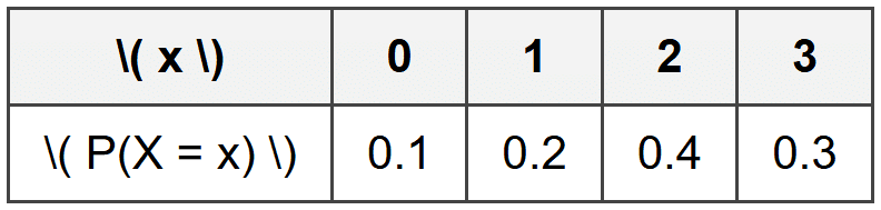
Example: A student takes a quiz where partial credit is possible.
Let \( X \) represent the score with this distribution:Find the variance and standard deviation of \( X \).
Solution:
First, find the expected value:
\( E(X) = (0)(0.1) + (1)(0.2) + (2)(0.4) + (3)(0.3) = 0 + 0.2 + 0.8 + 0.9 = 2.0 \)
Next, find \( E(X^2) \):
\( E(X^2) = (0^2)(0.1) + (1^2)(0.2) + (2^2)(0.4) + (3^2)(0.3) \)
\( E(X^2) = (0)(0.1) + (1)(0.2) + (4)(0.4) + (9)(0.3) = 0 + 0.2 + 1.6 + 2.7 = 4.5 \)
Now calculate the variance:
\( \text{Var}(X) = E(X^2) - [E(X)]^2 = 4.5 - (2.0)^2 = 4.5 - 4.0 = 0.5 \)
Finally, find the standard deviation:
\( \sigma = \sqrt{0.5} \approx 0.707 \)
The variance is 0.5 and the standard deviation is approximately 0.707 points.
Common Discrete Probability Distributions
While any valid assignment of probabilities to discrete values creates a probability distribution, certain patterns appear so frequently that they have special names and formulas. Understanding these standard distributions saves time and provides powerful tools for modeling real-world situations.
Discrete Uniform Distribution
The discrete uniform distribution occurs when all outcomes are equally likely. If a random variable \( X \) can take on \( n \) different values, and each value has the same probability, then \( X \) follows a discrete uniform distribution with:
\[ P(X = x) = \frac{1}{n} \]for each possible value of \( x \).
Rolling a fair die is a classic example: each of the six outcomes has probability \( \frac{1}{6} \). Drawing a card from a well-shuffled deck gives each card probability \( \frac{1}{52} \).
For a discrete uniform distribution with values \( 1, 2, 3, \ldots, n \), the expected value is:
\[ E(X) = \frac{n + 1}{2} \]This makes intuitive sense-the average of the numbers from 1 to \( n \) is the middle value.
Binomial Distribution (Brief Introduction)
The binomial distribution models situations where we perform a fixed number of independent trials, each trial has exactly two possible outcomes (success or failure), and the probability of success remains constant across trials.
A binomial random variable \( X \) represents the number of successes in \( n \) trials when the probability of success on each trial is \( p \). We write \( X \sim \text{Binomial}(n, p) \) to indicate that \( X \) follows a binomial distribution.
Examples include: the number of heads in 10 coin flips, the number of correct answers on a 20-question true/false test if you guess randomly, or the number of defective items in a sample of 50 products.
The probability formula for the binomial distribution is:
\[ P(X = k) = \binom{n}{k} p^k (1-p)^{n-k} \]where \( \binom{n}{k} = \frac{n!}{k!(n-k)!} \) is the binomial coefficient (read as "n choose k"), which counts the number of ways to choose \( k \) successes from \( n \) trials.
The expected value and variance of a binomial distribution are:
\[ E(X) = np \] \[ \text{Var}(X) = np(1-p) \]Example: A basketball player has a 70% free-throw success rate.
She attempts 5 free throws.
Let \( X \) represent the number of successful free throws.What is the probability she makes exactly 4 free throws?
Solution:
This is a binomial situation with \( n = 5 \) trials and \( p = 0.7 \) probability of success.
We want \( P(X = 4) \), so use the formula with \( k = 4 \):
\( P(X = 4) = \binom{5}{4} (0.7)^4 (0.3)^1 \)
\( \binom{5}{4} = \frac{5!}{4! \cdot 1!} = 5 \)
\( P(X = 4) = 5 \times (0.7)^4 \times (0.3) = 5 \times 0.2401 \times 0.3 = 5 \times 0.07203 = 0.36015 \)
The probability of making exactly 4 out of 5 free throws is approximately 0.360 or 36%.
Linear Transformations of Random Variables
Sometimes we need to transform a random variable by adding a constant, multiplying by a constant, or both. Understanding how these transformations affect the expected value and variance is crucial for practical applications.
Suppose \( X \) is a discrete random variable, and we create a new random variable \( Y \) by the linear transformation:
\[ Y = aX + b \]where \( a \) and \( b \) are constants. The following rules apply:
Effect on Expected Value
\[ E(Y) = E(aX + b) = aE(X) + b \]In words: the expected value of a linear transformation equals the transformation applied to the expected value. Multiplying by \( a \) multiplies the expected value by \( a \), and adding \( b \) adds \( b \) to the expected value.
Effect on Variance
\[ \text{Var}(Y) = \text{Var}(aX + b) = a^2 \text{Var}(X) \]Notice that adding a constant \( b \) does not change the variance-it only shifts all values by the same amount, which doesn't affect spread. Multiplying by \( a \) multiplies the variance by \( a^2 \) (not just \( a \)).
For standard deviation:
\[ \sigma_Y = |a| \sigma_X \]The standard deviation is multiplied by the absolute value of \( a \).
Example: A company measures employee productivity with a scoring system.
The raw score \( X \) has mean 50 and standard deviation 10.
To create a standardized score, they use the transformation \( Y = 2X + 30 \).What are the mean and standard deviation of \( Y \)?
Solution:
Given: \( E(X) = 50 \), \( \sigma_X = 10 \), and \( Y = 2X + 30 \)
Find the mean of \( Y \):
\( E(Y) = 2E(X) + 30 = 2(50) + 30 = 100 + 30 = 130 \)
Find the variance of \( Y \):
\( \text{Var}(Y) = 2^2 \text{Var}(X) = 4 \times 10^2 = 4 \times 100 = 400 \)
Find the standard deviation of \( Y \):
\( \sigma_Y = \sqrt{400} = 20 \)
The standardized score has mean 130 and standard deviation 20.
Working with Probability Calculations
Beyond finding probabilities for single values, we often need to find probabilities for ranges of values or combinations of events.
Cumulative Probability
The cumulative probability \( P(X \leq x) \) represents the probability that the random variable takes on a value less than or equal to \( x \). To find it, add up the probabilities for all values up to and including \( x \):
\[ P(X \leq x) = \sum_{k \leq x} P(X = k) \]Similarly, we can find probabilities for other ranges:
- \( P(X < x)="" \)="sum" of="" probabilities="" for="" all="" values="" strictly="" less="" than="" \(="" x="">
- \( P(X \geq x) \) = sum of probabilities for all values greater than or equal to \( x \)
- \( P(X > x) \) = sum of probabilities for all values strictly greater than \( x \)
- \( P(a \leq X \leq b) \) = sum of probabilities for all values from \( a \) to \( b \) inclusive
A useful relationship: since all probabilities sum to 1, we have:
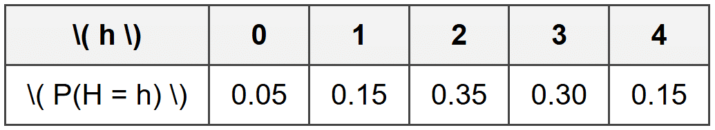
\[ P(X > x) = 1 - P(X \leq x) \]Example: A survey asks how many hours students spend on homework daily.
Let \( H \) represent hours with this distribution:Find the probability that a randomly selected student spends at least 2 hours on homework.
Solution:
We need \( P(H \geq 2) \), which includes \( H = 2, 3, \) or \( 4 \).
\( P(H \geq 2) = P(H = 2) + P(H = 3) + P(H = 4) \)
\( P(H \geq 2) = 0.35 + 0.30 + 0.15 = 0.80 \)
The probability is 0.80 or 80% that a student spends at least 2 hours on homework.
Independence and Joint Distributions
Sometimes we work with more than one random variable at a time. When two random variables \( X \) and \( Y \) are independent, knowing the value of one provides no information about the other. Mathematically, \( X \) and \( Y \) are independent if:
\[ P(X = x \text{ and } Y = y) = P(X = x) \cdot P(Y = y) \]for all possible pairs of values \( x \) and \( y \).
When random variables are independent, calculations become much simpler. For example, if \( X \) and \( Y \) are independent:
\[ E(X + Y) = E(X) + E(Y) \] \[ \text{Var}(X + Y) = \text{Var}(X) + \text{Var}(Y) \]The expected value rule actually holds whether or not the variables are independent, but the variance rule requires independence.
Think of rolling two dice simultaneously. The outcome on the first die doesn't affect the outcome on the second die-they're independent. If \( X \) is the number on the first die and \( Y \) is the number on the second die, then the sum \( X + Y \) has expected value \( E(X) + E(Y) = 3.5 + 3.5 = 7 \).
Applications and Practical Uses
Discrete random variables appear throughout science, business, social studies, and everyday decision-making:
- Quality Control: Manufacturers use discrete random variables to model the number of defective items in a batch, helping them determine inspection procedures and warranty costs.
- Insurance: Companies model the number of claims and claim amounts to set premiums and maintain profitability.
- Healthcare: Researchers track the number of patients who respond to a treatment, the number of hospital visits, or the number of symptoms present.
- Sports Analytics: Teams analyze discrete outcomes like points scored, turnovers, or successful plays to develop strategies.
- Marketing: Businesses model customer behavior, such as the number of purchases, website visits, or responses to advertising.
- Network Reliability: Engineers study the number of system failures or packet losses in communication networks.
Understanding discrete random variables equips you with tools to quantify uncertainty, make predictions based on probability, and make rational decisions when outcomes are not certain. Whether you're evaluating a business opportunity, interpreting survey results, or analyzing game strategies, the principles of discrete random variables provide a rigorous framework for working with randomness and chance.


