Chapter Notes: Transforming & Combining Random Variables


When we study real-world situations that involve randomness, we often need to work with multiple random variables at once. Sometimes we want to combine two random variables by adding or subtracting them. Other times, we want to transform a single random variable by multiplying it by a constant or adding a constant to it. Understanding how these operations affect the mean, variance, and standard deviation of random variables is essential for analyzing data and making predictions. In this chapter, we'll explore the rules and techniques for transforming and combining random variables, and we'll see how these tools help us model complex real-world scenarios.
Transforming a Single Random Variable
A transformation occurs when we apply a mathematical operation to every value of a random variable. The two most common transformations are adding (or subtracting) a constant and multiplying (or dividing) by a constant. These transformations change the distribution of the random variable in predictable ways.
Adding or Subtracting a Constant
When we add a constant to a random variable, we shift every value in the distribution by that constant amount. Suppose \( X \) is a random variable with mean \( \mu_X \) and standard deviation \( \sigma_X \). If we create a new random variable \( Y = X + c \), where \( c \) is a constant, the following rules apply:
- The mean shifts by the constant: \( \mu_Y = \mu_X + c \)
- The variance stays the same: \( \sigma_Y^2 = \sigma_X^2 \)
- The standard deviation stays the same: \( \sigma_Y = \sigma_X \)
Think of this like shifting everyone's test score by adding 5 bonus points. Everyone's score goes up by 5, so the average goes up by 5, but the spread of scores stays exactly the same.
Important Note: Adding or subtracting a constant changes the center of the distribution but does not change the spread. The standard deviation measures how far values typically are from the mean, and since we're moving all values by the same amount, their distances from each other remain unchanged.
Example: A coffee shop measures the temperature of their coffee in degrees Celsius.
The temperature \( X \) has a mean of 70°C and a standard deviation of 3°C.
They decide to report temperatures in a new scale where \( Y = X - 50 \).What are the mean and standard deviation of \( Y \)?
Solution:
We are subtracting 50 from every temperature value.
Mean of \( Y \): \( \mu_Y = \mu_X - 50 = 70 - 50 = 20 \)
Standard deviation of \( Y \): \( \sigma_Y = \sigma_X = 3 \)
The mean of the new temperature scale is 20 with a standard deviation of 3.
Multiplying or Dividing by a Constant
When we multiply a random variable by a constant, we stretch or compress the entire distribution. If \( Y = aX \), where \( a \) is a constant and \( X \) is a random variable, then:
- The mean is multiplied by that constant: \( \mu_Y = a\mu_X \)
- The variance is multiplied by the square of that constant: \( \sigma_Y^2 = a^2\sigma_X^2 \)
- The standard deviation is multiplied by the absolute value of that constant: \( \sigma_Y = |a|\sigma_X \)
Imagine measuring everyone's height in inches, then converting to centimeters by multiplying by 2.54. The average height gets multiplied by 2.54, and the standard deviation also gets multiplied by 2.54, making the distribution wider.
Important Note: When we multiply by a constant, both the center and the spread change. The variance is multiplied by \( a^2 \) because variance involves squared deviations from the mean. We use the absolute value for standard deviation because standard deviation is always non-negative, even if we multiply by a negative constant.
Example: A factory produces widgets whose weights \( X \) (in pounds) have a mean of 12 pounds and a standard deviation of 0.8 pounds.
Management wants to report weights in ounces, so they create \( Y = 16X \) (since 1 pound = 16 ounces).What are the mean and standard deviation of \( Y \)?
Solution:
We are multiplying every weight by 16.
Mean of \( Y \): \( \mu_Y = 16\mu_X = 16 × 12 = 192 \) ounces
Standard deviation of \( Y \): \( \sigma_Y = 16\sigma_X = 16 × 0.8 = 12.8 \) ounces
The mean weight in ounces is 192 ounces with a standard deviation of 12.8 ounces.
Combined Transformations
Often we need to both multiply and add constants to a random variable. If \( Y = aX + b \), we apply both rules in sequence:
\[ \mu_Y = a\mu_X + b \] \[ \sigma_Y = |a|\sigma_X \]Notice that the constant \( b \) affects only the mean, not the standard deviation. The multiplier \( a \) affects both the mean and the standard deviation.
Example: The time \( X \) (in hours) that students spend on homework each week has a mean of 8 hours and a standard deviation of 2 hours.
A researcher creates a new variable \( Y = 3X + 5 \) to model total study time including class time.What are the mean and standard deviation of \( Y \)?
Solution:
We apply the transformation \( Y = 3X + 5 \).
Mean of \( Y \): \( \mu_Y = 3\mu_X + 5 = 3(8) + 5 = 24 + 5 = 29 \) hours
Standard deviation of \( Y \): \( \sigma_Y = |3|\sigma_X = 3(2) = 6 \) hours
The mean of \( Y \) is 29 hours with a standard deviation of 6 hours.
Combining Two Random Variables by Addition or Subtraction
In many situations, we need to combine two different random variables. For example, we might want to know the total profit from two stores, or the difference in test scores between two groups. Understanding how to combine random variables is crucial for modeling these scenarios.
Rules for Means
The mean of a sum or difference of random variables follows a simple, intuitive rule. If \( X \) and \( Y \) are two random variables, then:
- For addition: \( \mu_{X+Y} = \mu_X + \mu_Y \)
- For subtraction: \( \mu_{X-Y} = \mu_X - \mu_Y \)
These rules always work, regardless of whether the random variables are independent or related. The mean of the sum is the sum of the means, and the mean of the difference is the difference of the means.
Rules for Variances: Independent Random Variables
When dealing with variance and standard deviation, we must be more careful. The key concept is independence. Two random variables are independent if knowing the value of one gives no information about the value of the other.
For independent random variables \( X \) and \( Y \):
- For addition: \( \sigma_{X+Y}^2 = \sigma_X^2 + \sigma_Y^2 \)
- For subtraction: \( \sigma_{X-Y}^2 = \sigma_X^2 + \sigma_Y^2 \)
Notice that we add variances even when subtracting random variables. This is because variance measures spread, and both addition and subtraction increase the potential spread of outcomes.
The standard deviation is the square root of the variance:
\[ \sigma_{X+Y} = \sqrt{\sigma_X^2 + \sigma_Y^2} \] \[ \sigma_{X-Y} = \sqrt{\sigma_X^2 + \sigma_Y^2} \]Important Note: We can only add variances when the random variables are independent. If the variables are related (for example, if high values of one tend to occur with high values of the other), we need more advanced techniques involving covariance.
Example: A delivery company has two drivers, Alice and Bob.
Alice's daily deliveries \( A \) have a mean of 25 packages with a standard deviation of 4 packages.
Bob's daily deliveries \( B \) have a mean of 30 packages with a standard deviation of 5 packages.
Assume their deliveries are independent.What are the mean and standard deviation of the total daily deliveries \( T = A + B \)?
Solution:
Mean of total deliveries: \( \mu_T = \mu_A + \mu_B = 25 + 30 = 55 \) packages
Variance of total deliveries: \( \sigma_T^2 = \sigma_A^2 + \sigma_B^2 = 4^2 + 5^2 = 16 + 25 = 41 \)
Standard deviation of total deliveries: \( \sigma_T = \sqrt{41} \approx 6.4 \) packages
The total daily deliveries have a mean of 55 packages and a standard deviation of approximately 6.4 packages.
Example: A manufacturing process involves two stages.
Stage 1 has a mean time of 12 minutes with a standard deviation of 2 minutes.
Stage 2 has a mean time of 18 minutes with a standard deviation of 3 minutes.
The stages are independent.What are the mean and standard deviation of the total processing time?
Solution:
Let \( X \) be the time for Stage 1 and \( Y \) be the time for Stage 2. Total time is \( T = X + Y \).
Mean total time: \( \mu_T = \mu_X + \mu_Y = 12 + 18 = 30 \) minutes
Variance of total time: \( \sigma_T^2 = \sigma_X^2 + \sigma_Y^2 = 2^2 + 3^2 = 4 + 9 = 13 \)
Standard deviation of total time: \( \sigma_T = \sqrt{13} \approx 3.6 \) minutes
The total processing time has a mean of 30 minutes and a standard deviation of approximately 3.6 minutes.
Understanding Why Variances Add
It may seem counterintuitive that we add variances even when subtracting random variables. Here's why this makes sense:
Variance measures uncertainty or variability. When we combine two independent sources of uncertainty, the total uncertainty increases. Even if we're subtracting one variable from another, we're still dealing with two sources of variability, so the total spread increases.
For example, if you measure your profit as revenue minus cost, and both revenue and cost are uncertain, your profit becomes even more uncertain than either component alone.
Example: A quality control inspector measures parts from two machines.
Machine X produces parts with a mean length of 50 mm and standard deviation of 1.2 mm.
Machine Y produces parts with a mean length of 48 mm and standard deviation of 0.9 mm.
The machines operate independently.What are the mean and standard deviation of the difference \( D = X - Y \)?
Solution:
Mean of the difference: \( \mu_D = \mu_X - \mu_Y = 50 - 48 = 2 \) mm
Variance of the difference: \( \sigma_D^2 = \sigma_X^2 + \sigma_Y^2 = (1.2)^2 + (0.9)^2 = 1.44 + 0.81 = 2.25 \)
Standard deviation of the difference: \( \sigma_D = \sqrt{2.25} = 1.5 \) mm
The difference in lengths has a mean of 2 mm and a standard deviation of 1.5 mm.
Combining More Than Two Random Variables
The same rules extend naturally when we combine more than two random variables. For independent random variables \( X_1, X_2, X_3, \ldots, X_n \):
The mean of the sum is:
\[ \mu_{X_1 + X_2 + \cdots + X_n} = \mu_{X_1} + \mu_{X_2} + \cdots + \mu_{X_n} \]The variance of the sum is:
\[ \sigma_{X_1 + X_2 + \cdots + X_n}^2 = \sigma_{X_1}^2 + \sigma_{X_2}^2 + \cdots + \sigma_{X_n}^2 \]The standard deviation is the square root of the variance.
Example: A restaurant tracks tips from three servers during lunch.
Server 1: mean = $45, standard deviation = $8
Server 2: mean = $52, standard deviation = $10
Server 3: mean = $38, standard deviation = $7
Assume tips are independent.What are the mean and standard deviation of total tips?
Solution:
Mean total tips: \( \mu = 45 + 52 + 38 = 135 \) dollars
Variance of total tips: \( \sigma^2 = 8^2 + 10^2 + 7^2 = 64 + 100 + 49 = 213 \)
Standard deviation of total tips: \( \sigma = \sqrt{213} \approx 14.6 \) dollars
The total tips have a mean of $135 and a standard deviation of approximately $14.60.
Linear Combinations of Random Variables
A linear combination occurs when we multiply random variables by constants and then add or subtract them. If we have \( W = aX + bY \), where \( a \) and \( b \) are constants and \( X \) and \( Y \) are independent random variables, then:
Mean of the linear combination:
\[ \mu_W = a\mu_X + b\mu_Y \]Variance of the linear combination:
\[ \sigma_W^2 = a^2\sigma_X^2 + b^2\sigma_Y^2 \]Standard deviation of the linear combination:
\[ \sigma_W = \sqrt{a^2\sigma_X^2 + b^2\sigma_Y^2} \]Notice that the coefficients \( a \) and \( b \) are squared when calculating variance. This follows from the rule that multiplying a random variable by a constant multiplies its variance by the square of that constant.
Example: A portfolio manager invests in two stocks.
Stock X: mean return = $120, standard deviation = $15
Stock Y: mean return = $80, standard deviation = $12
She creates a portfolio \( P = 2X + 3Y \) representing 2 shares of X and 3 shares of Y.
Assume the stocks are independent.What are the mean and standard deviation of the portfolio return?
Solution:
Mean portfolio return: \( \mu_P = 2\mu_X + 3\mu_Y = 2(120) + 3(80) = 240 + 240 = 480 \) dollars
Variance of portfolio: \( \sigma_P^2 = (2)^2\sigma_X^2 + (3)^2\sigma_Y^2 = 4(15)^2 + 9(12)^2 = 4(225) + 9(144) = 900 + 1296 = 2196 \)
Standard deviation of portfolio: \( \sigma_P = \sqrt{2196} \approx 46.9 \) dollars
The portfolio has a mean return of $480 with a standard deviation of approximately $46.90.
Special Case: Combining Identical Random Variables
A common situation involves combining multiple copies of the same random variable. For example, if we measure the same quantity multiple times, or if we sum the results from multiple identical trials.
If \( X_1, X_2, \ldots, X_n \) are \( n \) independent random variables, each with the same mean \( \mu \) and standard deviation \( \sigma \), then their sum \( S = X_1 + X_2 + \cdots + X_n \) has:
\[ \mu_S = n\mu \] \[ \sigma_S = \sqrt{n}\sigma \]The mean increases proportionally with \( n \), but the standard deviation increases only with the square root of \( n \). This is why averaging multiple measurements reduces uncertainty.
The sample mean \( \bar{X} = \frac{S}{n} = \frac{X_1 + X_2 + \cdots + X_n}{n} \) has:
\[ \mu_{\bar{X}} = \mu \] \[ \sigma_{\bar{X}} = \frac{\sigma}{\sqrt{n}} \]This shows that the mean of the sample mean equals the population mean, but the standard deviation decreases as sample size increases. This is a fundamental principle in statistics.
Example: A single dice roll has a mean of 3.5 and a standard deviation of approximately 1.71.
You roll the die 4 times independently and calculate the sum.What are the mean and standard deviation of the sum?
Solution:
We are summing 4 independent, identical random variables.
Mean of the sum: \( \mu_S = 4(3.5) = 14 \)
Standard deviation of the sum: \( \sigma_S = \sqrt{4}(1.71) = 2(1.71) = 3.42 \)
The sum of 4 dice rolls has a mean of 14 and a standard deviation of approximately 3.42.
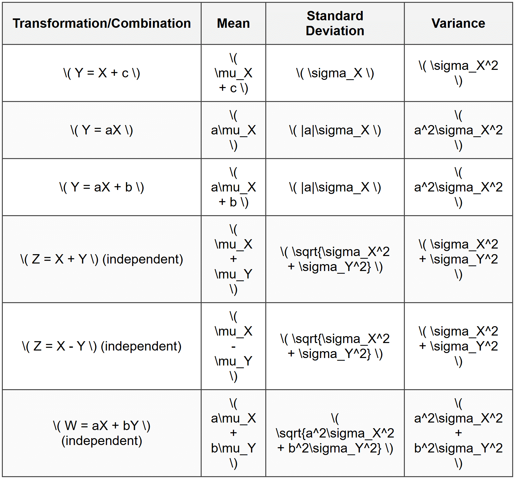
Summary of Transformation and Combination Rules
Here is a comprehensive table summarizing all the rules for transforming and combining random variables:
Practical Applications
Business and Finance
Companies frequently need to combine random variables when analyzing revenue, costs, and profits. If revenue and costs are both uncertain, the profit (revenue minus cost) has its own mean and standard deviation calculated using these rules. Portfolio managers use linear combinations to assess the risk and return of investments consisting of multiple assets.
Quality Control and Manufacturing
When multiple manufacturing processes contribute to a final product, engineers add the variances of each independent process to determine the total variation in the final product. This helps set quality control limits and predict defect rates.
Scientific Measurement
When scientists take multiple measurements of the same quantity, they calculate the mean to get a better estimate. The standard error (standard deviation of the mean) decreases with the square root of the number of measurements, providing more precise results.
Example: A restaurant calculates daily profit as \( P = R - C \), where \( R \) is revenue and \( C \) is cost.
Daily revenue: mean = $2400, standard deviation = $300
Daily cost: mean = $1600, standard deviation = $150
Revenue and cost are independent.What are the mean and standard deviation of daily profit?
Solution:
Mean profit: \( \mu_P = \mu_R - \mu_C = 2400 - 1600 = 800 \) dollars
Variance of profit: \( \sigma_P^2 = \sigma_R^2 + \sigma_C^2 = 300^2 + 150^2 = 90000 + 22500 = 112500 \)
Standard deviation of profit: \( \sigma_P = \sqrt{112500} \approx 335.4 \) dollars
The daily profit has a mean of $800 and a standard deviation of approximately $335.40.


