Chapter Notes: Geometric Random Variables


In many real-world situations, we repeat an action over and over until we succeed. Think about shooting free throws in basketball-you might miss the first few shots, but eventually you make one. Or consider inspecting items coming off an assembly line until you find one that's defective. In each case, we're counting the number of trials until something specific happens for the first time. This counting process can be modeled using what statisticians call a geometric random variable. Understanding geometric random variables helps us analyze situations where we're waiting for the first success in a sequence of independent trials.
What Is a Geometric Random Variable?
A geometric random variable counts the number of independent trials needed to get the first success. Each trial has only two possible outcomes-success or failure-and the probability of success remains the same from trial to trial. The key characteristic is that we stop as soon as we get our first success.
To qualify as a geometric setting, a situation must meet four specific conditions:
- Binary outcomes: Each trial results in either a success or a failure.
- Independent trials: The outcome of one trial does not affect the outcomes of other trials.
- Constant probability: The probability of success \( p \) remains the same for every trial.
- Counting until first success: We are interested in the number of trials until the first success occurs.
We typically use the letter \( X \) to represent the geometric random variable, and we write \( X \) ~ Geo(\( p \)) to indicate that \( X \) follows a geometric distribution with success probability \( p \).
Think of a geometric random variable like flipping a coin repeatedly until you get heads. If the coin is fair, \( p = 0.5 \). You might get heads on the first flip (\( X = 1 \)), or you might need 2 flips, 3 flips, or even more. The number of flips needed is your geometric random variable.
Probability Formula for Geometric Random Variables
If \( X \) is a geometric random variable with success probability \( p \), the probability that the first success occurs on the \( k \)th trial is given by:
\[ P(X = k) = (1 - p)^{k-1} \cdot p \]where:
- \( k \) = the trial number on which the first success occurs (1, 2, 3, ...)
- \( p \) = the probability of success on any single trial
- \( 1 - p \) = the probability of failure on any single trial
- \( (1 - p)^{k-1} \) = the probability of getting \( k - 1 \) failures before the success
The formula works because to get the first success on the \( k \)th trial, we must fail on the first \( k - 1 \) trials and then succeed on the \( k \)th trial. Since the trials are independent, we multiply these probabilities together.
Example: A basketball player has a 70% free throw success rate.
Each shot is independent of the others.What is the probability that the player makes her first free throw on the third attempt?
Solution:
Here, \( p = 0.7 \) and we want \( P(X = 3) \).
Using the formula: \( P(X = 3) = (1 - 0.7)^{3-1} \cdot 0.7 \)
\( P(X = 3) = (0.3)^2 \cdot 0.7 \)
\( P(X = 3) = 0.09 \cdot 0.7 = 0.063 \)
The probability that the player makes her first free throw on the third attempt is 0.063 or 6.3%.
Example: A quality control inspector examines computer chips.
Each chip has a 5% chance of being defective.
Chips are selected randomly and independently.What is the probability that the first defective chip is found on the first inspection?
Solution:
Here, \( p = 0.05 \) (success means finding a defective chip) and \( k = 1 \).
\( P(X = 1) = (1 - 0.05)^{1-1} \cdot 0.05 \)
\( P(X = 1) = (0.95)^0 \cdot 0.05 \)
\( P(X = 1) = 1 \cdot 0.05 = 0.05 \)
The probability that the first defective chip is found on the first inspection is 0.05 or 5%.
Cumulative Probability: Waiting At Most k Trials
Sometimes we want to know the probability that we'll get our first success within a certain number of trials. This is called a cumulative probability. To find \( P(X ≤ k) \), we can add up the individual probabilities for each value from 1 to \( k \).
However, there's a more efficient formula. The probability that the first success occurs within \( k \) trials is:
\[ P(X \leq k) = 1 - (1 - p)^k \]This formula uses the complement rule. The complement of "success within \( k \) trials" is "failure on all \( k \) trials," which has probability \( (1 - p)^k \).
Example: A student guesses randomly on a multiple-choice quiz.
Each question has 4 choices, so the probability of guessing correctly is 0.25.
Questions are answered independently.What is the probability the student guesses a correct answer within the first 3 attempts?
Solution:
Here, \( p = 0.25 \) and we want \( P(X ≤ 3) \).
Using the cumulative formula: \( P(X ≤ 3) = 1 - (1 - 0.25)^3 \)
\( P(X ≤ 3) = 1 - (0.75)^3 \)
\( P(X ≤ 3) = 1 - 0.421875 = 0.578125 \)
The probability that the student guesses correctly within the first 3 attempts is 0.578 or about 57.8%.
Probability of Waiting More Than k Trials
We might also want to calculate the probability that we need more than \( k \) trials to get the first success. This means we fail on all of the first \( k \) trials. The formula is straightforward:
\[ P(X > k) = (1 - p)^k \]This represents the probability of \( k \) consecutive failures.
Example: A archer hits the bullseye 40% of the time.
Each shot is independent.What is the probability that the archer needs more than 4 shots to hit the first bullseye?
Solution:
Here, \( p = 0.4 \) and we want \( P(X > 4) \).
Using the formula: \( P(X > 4) = (1 - 0.4)^4 \)
\( P(X > 4) = (0.6)^4 \)
\( P(X > 4) = 0.1296 \)
The probability that the archer needs more than 4 shots to hit the first bullseye is 0.1296 or about 13%.
Mean (Expected Value) of a Geometric Random Variable
The mean or expected value of a geometric random variable tells us the average number of trials we would need to get the first success if we repeated the process many times. For a geometric random variable with success probability \( p \), the mean is:
\[ \mu = E(X) = \frac{1}{p} \]where:
- \( \mu \) = the mean (expected number of trials)
- \( p \) = the probability of success on any single trial
This formula makes intuitive sense. If you have a 50% chance of success (\( p = 0.5 \)), you'd expect to need about \( \frac{1}{0.5} = 2 \) trials on average. If you have only a 10% chance (\( p = 0.1 \)), you'd expect to need about \( \frac{1}{0.1} = 10 \) trials.
Example: A factory machine produces bolts, and 2% of them are defective.
An inspector examines bolts one at a time until finding a defective one.On average, how many bolts must the inspector examine to find the first defective bolt?
Solution:
Here, \( p = 0.02 \).
The expected number of trials is: \( \mu = \frac{1}{p} = \frac{1}{0.02} \)
\( \mu = 50 \)
On average, the inspector must examine 50 bolts to find the first defective one.
Standard Deviation of a Geometric Random Variable
The standard deviation measures the typical spread or variability in the number of trials needed. For a geometric random variable, the variance is:
\[ \sigma^2 = \frac{1 - p}{p^2} \]And the standard deviation is the square root of the variance:
\[ \sigma = \sqrt{\frac{1 - p}{p^2}} = \frac{\sqrt{1 - p}}{p} \]where:
- \( \sigma^2 \) = the variance
- \( \sigma \) = the standard deviation
- \( p \) = the probability of success on any single trial
Example: A salesperson has a 20% success rate when cold-calling potential customers.
Each call is independent.Find the mean and standard deviation for the number of calls needed to make the first sale.
Solution:
Here, \( p = 0.20 \).
Mean: \( \mu = \frac{1}{0.20} = 5 \) calls
Standard deviation: \( \sigma = \frac{\sqrt{1 - 0.20}}{0.20} = \frac{\sqrt{0.80}}{0.20} \)
\( \sigma = \frac{0.894}{0.20} = 4.47 \) calls
On average, the salesperson needs 5 calls to make the first sale, with a standard deviation of about 4.47 calls.
The Memoryless Property
One of the most distinctive features of geometric random variables is the memoryless property. This property states that if we've already had several failures, the probability distribution for the number of additional trials needed doesn't depend on how many failures we've already experienced.
Mathematically, for a geometric random variable \( X \):
\[ P(X > m + n \mid X > m) = P(X > n) \]This means that if we've already waited \( m \) trials without success, the probability we'll need to wait at least \( n \) more trials is the same as if we were starting fresh.
Imagine flipping a coin until you get heads. Suppose you've flipped 5 times and gotten all tails. You might feel that heads is "due" to come up soon, but that's not how probability works. The memoryless property tells us that the coin doesn't remember the previous flips. The probability distribution for future flips is exactly the same as when you started.
Example: A gamer plays a game where the probability of winning any round is 0.3.
Rounds are independent.
The gamer has already lost 4 rounds in a row.What is the probability the gamer will need more than 3 additional rounds to get the first win?
Solution:
By the memoryless property, the previous 4 losses don't matter.
We simply calculate \( P(X > 3) \) where \( p = 0.3 \).
\( P(X > 3) = (1 - 0.3)^3 = (0.7)^3 \)
\( P(X > 3) = 0.343 \)
The probability of needing more than 3 additional rounds is 0.343 or 34.3%.
Distinguishing Geometric from Other Distributions
It's important to distinguish geometric random variables from similar probability models, particularly the binomial distribution.
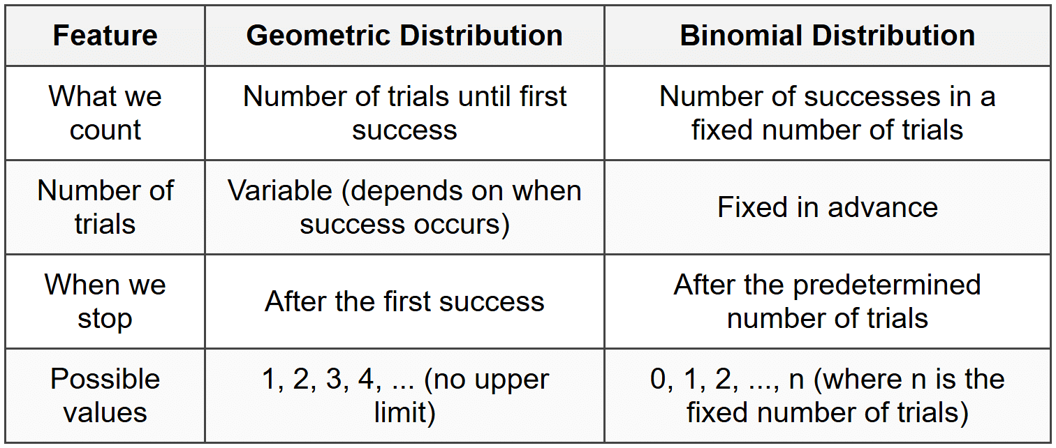
Binomial example: Flip a coin 10 times and count how many heads you get.
Geometric example: Flip a coin repeatedly until you get the first head, then count how many flips it took.
Real-World Applications
Geometric random variables appear in many practical contexts:
- Quality control: Testing items until finding the first defect
- Medical trials: Treating patients with a new therapy until the first patient responds positively
- Sports: Counting attempts until making the first successful shot, catch, or goal
- Marketing: Contacting potential customers until making the first sale
- Technology: Running software tests until encountering the first bug
- Environmental science: Sampling water from different locations until finding the first contaminated sample
Example: A pharmaceutical company tests a new drug.
Based on clinical trials, the drug is effective for 65% of patients.
Doctors will prescribe it to patients one at a time until finding the first patient who responds positively.What is the probability that exactly 2 patients need to be treated before finding the first positive response? What is the expected number of patients that will need treatment?
Solution:
Here, \( p = 0.65 \).
For the probability calculation: \( P(X = 2) = (1 - 0.65)^{2-1} \cdot 0.65 \)
\( P(X = 2) = (0.35)^1 \cdot 0.65 = 0.35 \cdot 0.65 = 0.2275 \)
For the expected value: \( \mu = \frac{1}{0.65} = 1.54 \) patients
The probability that exactly 2 patients need treatment is 0.2275 or 22.75%, and on average, 1.54 patients will need to be treated before finding the first positive response.
Common Mistakes and How to Avoid Them
When working with geometric random variables, students often make several common errors:
- Forgetting the exponent is k - 1, not k: Remember that we need \( k - 1 \) failures before the success on trial \( k \).
- Confusing "at least" and "at most": "At least \( k \) trials" means \( P(X ≥ k) \), while "at most \( k \) trials" means \( P(X ≤ k) \).
- Using the wrong probability for p: Make sure \( p \) represents the probability of the outcome you're calling "success" in your problem context.
- Forgetting the independence assumption: Geometric models only work when trials are truly independent.
- Mixing up geometric and binomial: Check whether you're counting trials until first success (geometric) or counting successes in a fixed number of trials (binomial).
Summary of Key Formulas
Here are the essential formulas for geometric random variables where \( X \) ~ Geo(\( p \)):
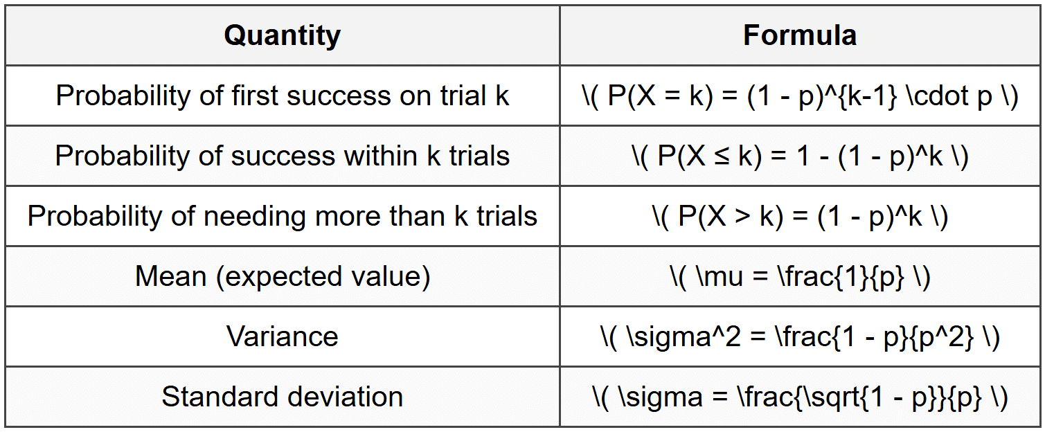
Understanding geometric random variables provides powerful tools for analyzing real-world situations where we're waiting for something to happen for the first time. By recognizing the geometric setting and applying these formulas correctly, you can answer important questions about how long you'll typically need to wait and how likely different waiting times are to occur.


