Chapter Notes: Poisson Distribution


The Poisson distribution is a powerful probability model used to describe the number of events occurring in a fixed interval of time or space. It is especially useful when we want to count rare or randomly scattered events-such as the number of customers arriving at a store in an hour, the number of phone calls received at a call center in a minute, or the number of typos on a printed page. Unlike the binomial distribution, which requires a fixed number of trials, the Poisson distribution works when we don't know how many opportunities for an event exist, only how often events typically occur. Understanding this distribution allows us to make predictions and informed decisions in fields ranging from business and healthcare to environmental science and engineering.
Characteristics of the Poisson Distribution
The Poisson distribution has several defining characteristics that make it distinct from other probability distributions:
- Counts of events: The random variable represents the number of times an event happens within a specific interval. This count must be a whole number (0, 1, 2, 3, and so on).
- Fixed interval: Events are counted over a fixed period of time, area, volume, or distance. For example, we might count arrivals in one hour or defects per square meter.
- Independence: Events occur independently of one another. The occurrence of one event does not affect the probability of another event happening.
- Constant average rate: Events occur at a constant average rate throughout the interval, denoted by the Greek letter lambda (\( \lambda \)). This rate represents the expected number of events per interval.
- Rare events: The Poisson distribution is most appropriate when events are relatively rare compared to the number of possible opportunities for them to occur.
These characteristics ensure that the Poisson model accurately reflects real-world scenarios where events happen sporadically but at a predictable average rate.
The Poisson Probability Formula
The probability of observing exactly \( k \) events in an interval, given an average rate of \( \lambda \) events per interval, is calculated using the Poisson probability mass function:
\[ P(X = k) = \frac{\lambda^k e^{-\lambda}}{k!} \]In this formula:
- \( X \) is the random variable representing the number of events
- \( k \) is the specific number of events we want to find the probability for (where \( k = 0, 1, 2, 3, \ldots \))
- \( \lambda \) (lambda) is the average number of events occurring in the interval
- \( e \) is Euler's number, approximately equal to 2.71828
- \( k! \) (k factorial) means \( k \times (k-1) \times (k-2) \times \ldots \times 2 \times 1 \), with the special case that \( 0! = 1 \)
This formula tells us the likelihood of any specific count occurring when we know the average rate. The term \( e^{-\lambda} \) ensures that all probabilities sum to 1 across all possible values of \( k \).
Example: A customer service center receives an average of 3 calls per minute.
Assume calls arrive independently and at a constant average rate.What is the probability that exactly 2 calls arrive in a given minute?
Solution:
We identify that \( \lambda = 3 \) calls per minute and we want to find \( P(X = 2) \).
Using the Poisson formula with \( k = 2 \):
\( P(X = 2) = \frac{3^2 \times e^{-3}}{2!} \)
Calculate the numerator: \( 3^2 = 9 \) and \( e^{-3} \approx 0.0498 \), so \( 9 \times 0.0498 \approx 0.4482 \)
Calculate the denominator: \( 2! = 2 \times 1 = 2 \)
Divide: \( P(X = 2) = \frac{0.4482}{2} = 0.2241 \)
The probability of receiving exactly 2 calls in a given minute is approximately 0.224 or 22.4%.
Example: A hospital emergency room sees an average of 4 patients per hour during the night shift.
What is the probability that exactly 5 patients arrive in a particular hour?
Solution:
Here \( \lambda = 4 \) patients per hour and we seek \( P(X = 5) \).
Apply the Poisson formula:
\( P(X = 5) = \frac{4^5 \times e^{-4}}{5!} \)
Calculate \( 4^5 = 1024 \)
Calculate \( e^{-4} \approx 0.0183 \)
Multiply: \( 1024 \times 0.0183 \approx 18.739 \)
Calculate \( 5! = 5 \times 4 \times 3 \times 2 \times 1 = 120 \)
Divide: \( P(X = 5) = \frac{18.739}{120} \approx 0.1562 \)
The probability of exactly 5 patients arriving in that hour is approximately 0.156 or 15.6%.
Mean and Variance
One of the elegant features of the Poisson distribution is the relationship between its mean and variance. Both the mean (expected value) and the variance of a Poisson distribution equal \( \lambda \):
\[ \text{Mean} = E(X) = \lambda \] \[ \text{Variance} = \text{Var}(X) = \lambda \]The standard deviation, which measures the typical spread of values around the mean, is the square root of the variance:
\[ \text{Standard Deviation} = \sigma = \sqrt{\lambda} \]This property simplifies many calculations. If we know the average rate \( \lambda \), we immediately know both how many events we expect on average and how much variability to expect around that average.
Think of it this way: if a bakery sells an average of 16 loaves of specialty bread per day, the mean number sold is 16 loaves. The variance is also 16, and the standard deviation is \( \sqrt{16} = 4 \) loaves. This tells us that while 16 is typical, the daily count usually varies by about 4 loaves in either direction.
Calculating Cumulative Probabilities
Often we need to find the probability of a range of outcomes rather than one exact value. Cumulative probabilities answer questions like "What is the probability of at most 3 events?" or "What is the probability of more than 2 events?"
The cumulative distribution function (CDF) gives the probability of observing \( k \) or fewer events:
\[ P(X \leq k) = \sum_{i=0}^{k} \frac{\lambda^i e^{-\lambda}}{i!} \]This means we add up the individual probabilities for \( X = 0, X = 1, X = 2, \ldots, X = k \).
To find probabilities for other ranges, we use these relationships:
- At least \( k \) events: \( P(X \geq k) = 1 - P(X \leq k-1) \)
- More than \( k \) events: \( P(X > k) = 1 - P(X \leq k) \)
- Fewer than \( k \) events: \( P(X < k)="P(X" \leq="" k-1)="">
- Between \( a \) and \( b \) events (inclusive): \( P(a \leq X \leq b) = P(X \leq b) - P(X \leq a-1) \)
Example: A website experiences an average of 2 crashes per week.
Assume crashes occur independently and randomly throughout the week.What is the probability of at most 1 crash in a given week?
Solution:
We have \( \lambda = 2 \) and need \( P(X \leq 1) = P(X = 0) + P(X = 1) \).
Calculate \( P(X = 0) = \frac{2^0 \times e^{-2}}{0!} = \frac{1 \times 0.1353}{1} = 0.1353 \)
Calculate \( P(X = 1) = \frac{2^1 \times e^{-2}}{1!} = \frac{2 \times 0.1353}{1} = 0.2706 \)
Add the probabilities: \( P(X \leq 1) = 0.1353 + 0.2706 = 0.4059 \)
The probability of at most 1 crash in a week is approximately 0.406 or 40.6%.
Example: A rare bird species is spotted an average of 1.5 times per month at a wildlife preserve.
What is the probability of seeing this bird more than 2 times in a given month?
Solution:
We have \( \lambda = 1.5 \) and need \( P(X > 2) = 1 - P(X \leq 2) \).
First find \( P(X \leq 2) = P(X = 0) + P(X = 1) + P(X = 2) \).
Calculate \( P(X = 0) = \frac{1.5^0 \times e^{-1.5}}{0!} = e^{-1.5} \approx 0.2231 \)
Calculate \( P(X = 1) = \frac{1.5^1 \times e^{-1.5}}{1!} = 1.5 \times 0.2231 \approx 0.3347 \)
Calculate \( P(X = 2) = \frac{1.5^2 \times e^{-1.5}}{2!} = \frac{2.25 \times 0.2231}{2} \approx 0.2510 \)
Sum these: \( P(X \leq 2) = 0.2231 + 0.3347 + 0.2510 = 0.8088 \)
Therefore, \( P(X > 2) = 1 - 0.8088 = 0.1912 \)
The probability of seeing the bird more than 2 times in a month is approximately 0.191 or 19.1%.
Adjusting the Interval
The value of \( \lambda \) depends on the length or size of the interval we're considering. If we know the average rate per unit interval, we can scale \( \lambda \) proportionally to match a different interval.
If events occur at an average rate of \( r \) per unit interval, then for an interval of length \( t \), the parameter becomes:
\[ \lambda = r \times t \]This flexibility allows us to answer questions about different time periods or spatial regions using the same underlying rate.
Example: A factory machine produces defective items at an average rate of 0.5 defects per hour.
The machine operates continuously.What is the probability of exactly 3 defects occurring in a 4-hour shift?
Solution:
The rate is \( r = 0.5 \) defects per hour, and the interval is \( t = 4 \) hours.
Calculate \( \lambda = 0.5 \times 4 = 2 \) defects per 4-hour shift.
Now find \( P(X = 3) \) with \( \lambda = 2 \):
\( P(X = 3) = \frac{2^3 \times e^{-2}}{3!} = \frac{8 \times 0.1353}{6} = \frac{1.0824}{6} \approx 0.1804 \)
The probability of exactly 3 defects in a 4-hour shift is approximately 0.180 or 18.0%.
Poisson Approximation to the Binomial
The Poisson distribution can be used to approximate the binomial distribution when certain conditions are met. Specifically, when the number of trials \( n \) is large and the probability of success \( p \) is small, the binomial distribution \( \text{Binomial}(n, p) \) closely resembles a Poisson distribution with \( \lambda = np \).
The general rule of thumb is to use the Poisson approximation when:
- \( n \geq 100 \)
- \( p \leq 0.01 \)
- \( np \leq 10 \)
This approximation simplifies calculations significantly, as computing binomial probabilities with large \( n \) can be tedious, while Poisson probabilities remain straightforward regardless of the rate.
Example: A quality control inspector examines 200 manufactured parts.
Historical data shows that 0.5% of parts are defective.What is the approximate probability that exactly 2 defective parts are found?
Solution:
This is a binomial situation with \( n = 200 \) and \( p = 0.005 \), but we can use the Poisson approximation.
Calculate \( \lambda = np = 200 \times 0.005 = 1 \).
Use the Poisson formula with \( \lambda = 1 \) and \( k = 2 \):
\( P(X = 2) = \frac{1^2 \times e^{-1}}{2!} = \frac{1 \times 0.3679}{2} = \frac{0.3679}{2} \approx 0.1839 \)
The probability of finding exactly 2 defective parts is approximately 0.184 or 18.4%.
Applications of the Poisson Distribution
The Poisson distribution appears in a wide variety of real-world contexts across many disciplines:
Business and Operations
- Modeling the number of customers arriving at a service counter during a specified time period
- Predicting the number of calls received at a customer service center per hour
- Estimating the number of claims filed with an insurance company each day
- Forecasting the number of website hits or server requests per second
Healthcare and Medicine
- Analyzing the number of patients arriving at an emergency room per shift
- Studying the incidence of rare diseases in a population over a year
- Modeling the number of mutations occurring in a DNA sequence
Environmental Science
- Counting the number of animals spotted in a wildlife survey area
- Measuring radioactive decay events detected by a Geiger counter per minute
- Tracking the number of earthquakes occurring in a region per month
Manufacturing and Quality Control
- Monitoring the number of defects per batch or per unit area in production
- Analyzing the number of accidents occurring in a factory per quarter
Technology and Communication
- Modeling network packet arrivals per millisecond
- Predicting the number of system failures or crashes per week
- Analyzing typos or errors per page in a document
In each of these cases, the Poisson distribution provides a mathematical framework for understanding randomness and making probabilistic predictions that inform decision-making.
Important Assumptions and Limitations
While the Poisson distribution is versatile, it relies on specific assumptions that must be checked before applying it:
- Independence: Events must occur independently. If one event influences the likelihood of another, the Poisson model may not be appropriate. For example, customer arrivals may not be independent if one customer tells friends about a sale, causing a rush.
- Constant rate: The average rate \( \lambda \) must remain constant throughout the interval. If the rate changes over time (such as more customers arriving during lunch hour than early morning), the simple Poisson model doesn't apply without adjustment.
- Non-simultaneous events: The probability of two or more events occurring at exactly the same instant must be negligible. In practice, we assume events are separated in time or space.
- Single parameter: The Poisson distribution is fully determined by one parameter, \( \lambda \). This means the mean equals the variance, which may not hold in all real-world data. If observed variance greatly exceeds the mean, a different model (such as the negative binomial distribution) may be more suitable.
Before using the Poisson distribution, verify these conditions are reasonably met in your context. When assumptions are violated, the resulting probabilities may be inaccurate, leading to poor predictions or decisions.
Using Technology for Poisson Calculations
While the Poisson formula can be computed by hand for small values of \( k \) and \( \lambda \), technology greatly simplifies calculations, especially for cumulative probabilities or large parameter values. Most statistical software, graphing calculators, and spreadsheet programs include built-in functions for the Poisson distribution.
Common Tools and Functions
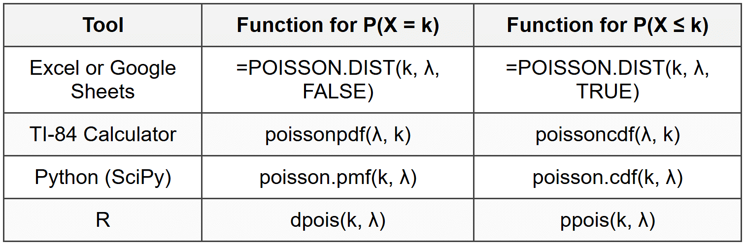
Using these tools, you can quickly explore probabilities for various scenarios, validate hand calculations, and analyze larger datasets efficiently.
Summary of Key Formulas
Here is a concise reference for the essential formulas related to the Poisson distribution:
- Probability mass function: \( P(X = k) = \frac{\lambda^k e^{-\lambda}}{k!} \)
- Mean: \( E(X) = \lambda \)
- Variance: \( \text{Var}(X) = \lambda \)
- Standard deviation: \( \sigma = \sqrt{\lambda} \)
- Cumulative probability: \( P(X \leq k) = \sum_{i=0}^{k} \frac{\lambda^i e^{-\lambda}}{i!} \)
- Scaling for different intervals: \( \lambda = r \times t \), where \( r \) is the rate per unit and \( t \) is the interval length
Mastering these formulas and understanding when to apply them equips you to model and analyze count data in diverse practical situations. The Poisson distribution is a foundational tool in probability and statistics, bridging theoretical concepts with real-world problem solving.


