Chapter Notes: Significance Tests (Hypothesis Testing)

Table of Contents
1. The Logic of Hypothesis Testing
2. Setting Up Hypotheses
3. Test Statistics
4. P-Values
5. Significance Level and Decision Rules
6. Types of Errors
7. Conditions for Valid Significance Tests
8. Complete Hypothesis Test Procedure
9. Statistical Significance vs. Practical Importance
10. One-Sample and Two-Sample Tests
11. Connecting Confidence Intervals and Hypothesis Tests
View more

When scientists make a discovery, when doctors test a new medicine, or when companies analyze customer behavior, they all face the same fundamental question: Is what I'm observing real, or could it just be due to random chance? Significance tests, also called hypothesis tests, give us a formal way to answer this question using data and probability. In a significance test, we start with a claim about a population, collect sample data, and then determine whether the data provides convincing evidence against that claim. This powerful statistical method helps us make decisions and draw conclusions when we can't measure an entire population.

The Logic of Hypothesis Testing

Hypothesis testing works by assuming something is true and then checking whether our data contradicts that assumption. Think of it like a court trial: we assume the defendant is innocent (our initial claim) and then examine the evidence to see if it's strong enough to reject that assumption. If the evidence is very unlikely under the assumption of innocence, we conclude the defendant is guilty. Similarly, in hypothesis testing, if our data would be very unlikely under our initial assumption, we reject that assumption.

Every significance test involves two competing hypotheses:

• Null Hypothesis (H₀): This is the claim we assume to be true at the start. It usually represents "no effect," "no difference," or "no change" from a known value. The null hypothesis always contains an equality (=, ≤, or ≥).
• Alternative Hypothesis (Hₐ or H₁): This is the claim we're trying to find evidence for. It represents "there is an effect," "there is a difference," or "there has been a change." The alternative hypothesis contains an inequality (<,>, or ≠).

The null hypothesis is what we test directly. We never "prove" the null hypothesis; we either reject it (if evidence is strong) or fail to reject it (if evidence is weak).

Setting Up Hypotheses

The first step in any significance test is to clearly state both hypotheses. The way we write them depends on what question we're investigating.

One-Sided Tests (One-Tailed Tests)

A one-sided test looks for evidence of a change in a specific direction. We use a one-sided test when we only care whether a parameter is greater than or less than a certain value, not both.

Right-tailed test (testing if a parameter is greater than a value):

where \( \mu \) represents the population parameter and \( \mu_0 \) represents the claimed value.

Left-tailed test (testing if a parameter is less than a value):

Two-Sided Tests (Two-Tailed Tests)

A two-sided test looks for evidence of any difference from the claimed value, regardless of direction. We use a two-sided test when we care whether a parameter is different (either higher or lower) from a certain value.

Example:  A coffee company claims their bags contain 16 ounces of coffee on average.
A consumer advocacy group suspects the bags contain less than advertised.

What are the appropriate hypotheses?

Solution:

Let \( \mu \) = the true mean weight of coffee bags in ounces.

Since the group suspects bags contain less than advertised, this is a left-tailed test.

\( H_0: \mu = 16 \) (the company's claim is true)

\( H_a: \mu < 16="" \)="" (bags="" contain="" less="" than="">

The null hypothesis states the company's claim, and the alternative hypothesis represents what the advocacy group suspects: H₀: μ = 16 and Hₐ: μ <>.

Test Statistics

Once we have our hypotheses, we collect data and calculate a test statistic. A test statistic is a single number computed from sample data that measures how far our sample result is from what the null hypothesis predicts. Different situations require different test statistics.

Z-Test Statistic

When we know the population standard deviation \( \sigma \) or when we're working with proportions, we often use a z-test statistic:

For a population mean:

where \( \bar{x} \) is the sample mean, \( \mu_0 \) is the claimed population mean, \( \sigma \) is the population standard deviation, and \( n \) is the sample size.

For a population proportion:

where \( \hat{p} \) is the sample proportion, \( p_0 \) is the claimed population proportion, and \( n \) is the sample size.

T-Test Statistic

When we don't know the population standard deviation and must estimate it from our sample, we use a t-test statistic:

where \( s \) is the sample standard deviation. The t-statistic follows a t-distribution with \( n - 1 \) degrees of freedom.

The test statistic tells us how many standard errors our sample result is from the null hypothesis value. A larger absolute value indicates stronger evidence against the null hypothesis.

P-Values

The p-value is the probability of obtaining a test statistic at least as extreme as the one we calculated, assuming the null hypothesis is true. In plain English: If the null hypothesis were actually true, what's the chance we'd see data this unusual or more unusual?

The p-value quantifies the strength of evidence against the null hypothesis:

• A small p-value (typically ≤ 0.05) indicates strong evidence against H₀
• A large p-value (typically > 0.05) indicates weak evidence against H₀

How we calculate the p-value depends on whether our test is one-sided or two-sided:

• Right-tailed test: p-value = P(test statistic ≥ observed value)
• Left-tailed test: p-value = P(test statistic ≤ observed value)
• Two-tailed test: p-value = 2 × P(test statistic ≥ |observed value|)

Example:  A teacher claims that students in her class spend an average of 2 hours per night on homework.
A random sample of 25 students has a mean of 2.4 hours with a standard deviation of 0.8 hours.
Test at the 0.05 significance level whether students actually spend more than 2 hours.

Is there evidence that students spend more than 2 hours on homework?

Solution:

Step 1: State the hypotheses.
Let \( \mu \) = true mean homework time
\( H_0: \mu = 2 \)
\( H_a: \mu > 2 \) (right-tailed test)

Step 2: Calculate the test statistic.
Since \( \sigma \) is unknown, use a t-test:
\( t = \frac{2.4 - 2}{0.8 / \sqrt{25}} = \frac{0.4}{0.8/5} = \frac{0.4}{0.16} = 2.5 \)

Step 3: Find the p-value.
With df = 25 - 1 = 24 degrees of freedom and t = 2.5
Using a t-table or calculator: p-value ≈ 0.0098

Step 4: Make a decision.
Since p-value (0.0098) < α="" (0.05),="" we="" reject="">

There is convincing evidence that students spend more than 2 hours per night on homework.

Significance Level and Decision Rules

The significance level, denoted by \( \alpha \) (alpha), is a threshold we set before conducting the test. It represents the probability of rejecting the null hypothesis when it's actually true (a Type I error). Common significance levels are 0.10, 0.05, and 0.01, with 0.05 being most common.

The decision rule is straightforward:

• If p-value ≤ \( \alpha \): Reject H₀ (we have statistically significant results)
• If p-value > \( \alpha \): Fail to reject H₀ (we do not have statistically significant results)

Important note: "Fail to reject H₀" does NOT mean "accept H₀" or "prove H₀ is true." It simply means we don't have enough evidence to conclude H₀ is false.

Types of Errors

Because we're making decisions based on sample data rather than complete population information, we can make mistakes. There are two types of errors in hypothesis testing:

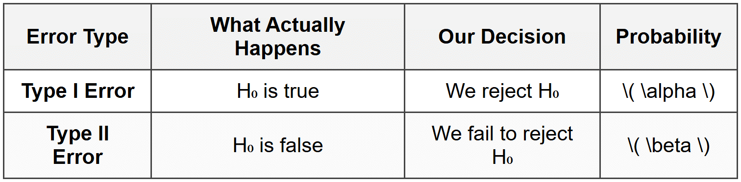
Type I Error: Rejecting a true null hypothesis (a "false alarm"). The probability of a Type I error equals the significance level \( \alpha \).

Type II Error: Failing to reject a false null hypothesis (a "missed detection"). The probability of a Type II error is denoted \( \beta \).

The power of a test is \( 1 - \beta \), which represents the probability of correctly rejecting a false null hypothesis. A more powerful test is better at detecting real effects.

Think of a smoke detector: A Type I error is when it goes off even though there's no fire (false alarm). A Type II error is when there's a fire but the detector doesn't go off (missed detection). We want to minimize both types of errors, but reducing one often increases the other.

Conditions for Valid Significance Tests

For our test results to be valid, certain conditions must be met. We check these before conducting the test.

Conditions for Tests About Means

• Random: The data must come from a random sample or randomized experiment
• Normal: The sampling distribution of \( \bar{x} \) must be approximately normal:
  • The population distribution is normal, OR
  • The sample size is large (n ≥ 30 by the Central Limit Theorem), OR
  • For smaller samples, the population distribution should be roughly symmetric with no strong outliers
• Independent: Individual observations must be independent. When sampling without replacement, the sample size should be less than 10% of the population size (the 10% condition)

Conditions for Tests About Proportions

• Random: The data must come from a random sample or randomized experiment
• Normal: The sampling distribution of \( \hat{p} \) must be approximately normal. Check that \( np_0 \geq 10 \) and \( n(1-p_0) \geq 10 \)
• Independent: Individual observations must be independent. When sampling without replacement, check the 10% condition: \( n \leq 0.10N \)

Complete Hypothesis Test Procedure

A well-structured hypothesis test follows these steps:

1. STATE: Define the parameter, state the hypotheses, and identify the significance level
2. PLAN: Name the test, check all conditions for using the test
3. DO: Calculate the test statistic and p-value
4. CONCLUDE: Make a decision and state your conclusion in context

Example:  A pharmaceutical company claims that 75% of patients experience relief from headaches within 30 minutes of taking their new medication.
In a random sample of 200 patients, 140 experienced relief within 30 minutes.
Test at the 0.05 significance level whether the true proportion is less than the company's claim.

Does the data provide evidence that the true proportion is less than 75%?

Solution:

STATE:
Parameter: p = the true proportion of all patients who experience relief within 30 minutes
\( H_0: p = 0.75 \)
\( H_a: p < 0.75="">
\( \alpha = 0.05 \)

PLAN:
One-sample z-test for a proportion
Random: The problem states this is a random sample ✓
Normal: \( np_0 = 200(0.75) = 150 \geq 10 \) and \( n(1-p_0) = 200(0.25) = 50 \geq 10 \) ✓
Independent: 200 is surely less than 10% of all potential patients ✓

DO:
Sample proportion: \( \hat{p} = 140/200 = 0.70 \)
Test statistic: \( z = \frac{0.70 - 0.75}{\sqrt{\frac{0.75(0.25)}{200}}} = \frac{-0.05}{\sqrt{0.0009375}} = \frac{-0.05}{0.0306} \approx -1.63 \)
P-value: P(Z < -1.63)="" ≈="">

CONCLUDE:
Since p-value (0.0516) > \( \alpha \) (0.05), we fail to reject H₀.
We do not have sufficient evidence at the 0.05 significance level to conclude that the true proportion of patients experiencing relief is less than 75%.

Statistical Significance vs. Practical Importance

An important distinction exists between statistical significance and practical importance. A result can be statistically significant (p-value < \(="" \alpha="" \))="" but="" not="" practically="" important,="" especially="" with="" very="" large="" sample="">

For example, a company might find that a new website design increases average time on site from 5.0 minutes to 5.1 minutes, and with a sample of 10,000 users, this difference might be statistically significant (p < 0.05).="" however,="" a="" 0.1-minute="" increase="" may="" not="" be="" practically="" meaningful="" for="" the="" company's="" business="">

Conversely, a result might fail to reach statistical significance (p-value > \( \alpha \)) but suggest a practically important effect. This often happens with small sample sizes where the test lacks sufficient power to detect real differences.

Always consider both statistical significance and practical importance when interpreting results. Ask yourself: Even if this result is real, does it matter in the real world?

One-Sample and Two-Sample Tests

One-Sample Tests

A one-sample test compares a sample statistic to a hypothesized population parameter. All the examples above have been one-sample tests. We use these when we want to know if our sample provides evidence that a population parameter differs from a claimed value.

Two-Sample Tests

A two-sample test compares statistics from two different samples to see if they come from populations with different parameters. For example, we might compare mean test scores between two teaching methods or compare proportions of defective products from two factories.

For two proportions, the hypotheses are:

The test statistic for two proportions is:

where \( \hat{p}_c = \frac{x_1 + x_2}{n_1 + n_2} \) is the combined (pooled) sample proportion.

For two means, when population standard deviations are unknown, we use a two-sample t-test with the test statistic:

Example:  A researcher wants to compare reading comprehension between two teaching methods.
Method A: 40 students, mean score = 78, standard deviation = 12
Method B: 35 students, mean score = 72, standard deviation = 10
Test at α = 0.05 whether Method A produces higher mean scores than Method B.

Is there evidence that Method A is more effective?

Solution:

STATE:
Parameters: \( \mu_1 \) = mean score for Method A, \( \mu_2 \) = mean score for Method B
\( H_0: \mu_1 = \mu_2 \) (or \( \mu_1 - \mu_2 = 0 \))
\( H_a: \mu_1 > \mu_2 \) (or \( \mu_1 - \mu_2 > 0 \))
\( \alpha = 0.05 \)

PLAN:
Two-sample t-test for means
Assuming random assignment to methods and both sample sizes are reasonably large (≥30 or ≥40)

DO:
\( t = \frac{78 - 72}{\sqrt{\frac{144}{40} + \frac{100}{35}}} = \frac{6}{\sqrt{3.6 + 2.857}} = \frac{6}{\sqrt{6.457}} = \frac{6}{2.541} \approx 2.36 \)
Using technology with df ≈ 34: p-value ≈ 0.012

CONCLUDE:
Since p-value (0.012) < α="" (0.05),="" we="" reject="">
There is convincing evidence that Method A produces higher mean reading comprehension scores than Method B.

Connecting Confidence Intervals and Hypothesis Tests

Confidence intervals and two-sided hypothesis tests are closely related. A two-sided hypothesis test at significance level \( \alpha \) will reject H₀ if and only if the hypothesized parameter value falls outside a \( (1-\alpha) \times 100\% \) confidence interval.

For example, if a 95% confidence interval for \( \mu \) is (52, 68), then a two-sided test of \( H_0: \mu = 70 \) at \( \alpha = 0.05 \) would reject H₀ because 70 falls outside the interval. However, a test of \( H_0: \mu = 60 \) would fail to reject H₀ because 60 falls inside the interval.

This connection provides a useful way to think about hypothesis tests: we're asking whether the claimed value is a plausible value for the parameter based on our sample data.