Chapter Notes: Inference About Slope

Table of Contents
1. The Regression Model and Conditions
2. Sampling Distribution of the Slope
3. Hypothesis Test for the Slope
4. Confidence Interval for the Slope
5. Interpreting Computer Output
6. Common Misconceptions and Important Notes
7. Connecting Hypothesis Tests and Confidence Intervals
8. Practical Steps for Performing Inference About Slope
9. Summary
View more

When we study the relationship between two quantitative variables, we often use a scatterplot and fit a least-squares regression line to summarize the data. The slope of that line tells us how much the response variable changes, on average, for each one-unit increase in the explanatory variable. But here's an important question: when we calculate a slope from a sample of data, how confident can we be that the true relationship in the entire population isn't just zero? In other words, is there really a relationship between the variables, or could the pattern we see be due to chance alone? Inference about slope means using sample data to make conclusions about the true slope in the population. This process involves creating confidence intervals for the slope and performing hypothesis tests to determine whether the slope is statistically significant.

The Regression Model and Conditions

Before we can perform inference about the slope of a regression line, we need to establish the underlying model and check that certain conditions are met. When we collect data on two variables and fit a regression line, we're working with a sample. Our goal is to say something about the true relationship in the entire population.

The Population Regression Model

In the population, we assume there is a true linear relationship between the explanatory variable \( x \) and the response variable \( y \). This relationship can be written as:

Here, \( \alpha \) (alpha) is the true y-intercept in the population, \( \beta \) (beta) is the true slope in the population, and \( \epsilon \) (epsilon) is the error term or residual. The error term represents the random variation in \( y \) that isn't explained by the linear relationship with \( x \). We assume that for any fixed value of \( x \), the error terms are normally distributed with mean zero and constant standard deviation \( \sigma \).

When we collect a sample and calculate the least-squares regression line, we get estimates of these population parameters. The sample slope is denoted \( b \) and estimates \( \beta \). The sample y-intercept is denoted \( a \) and estimates \( \alpha \).

Conditions for Inference

To perform valid inference about the slope, we must verify four important conditions. You can remember them with the acronym LINE:

• Linear: The relationship between \( x \) and \( y \) must be linear. Check this by looking at a scatterplot of the data. The points should show a roughly straight pattern, not a curve.
• Independent: The observations must be independent of one another. This is usually satisfied if the data come from a random sample or a randomized experiment. A common rule is that the sample size should be less than 10% of the population size.
• Normal: For any fixed value of \( x \), the response values (or the residuals) should be normally distributed. Check this by making a histogram or normal probability plot of the residuals. They should be approximately symmetric and bell-shaped.
• Equal variance: The variability of the response values should be roughly the same for all values of \( x \). Check this by looking at a residual plot (residuals versus \( x \) or versus predicted values). The vertical spread of points should be roughly constant across the plot, with no fan or cone shape.

If any of these conditions are clearly violated, the inference procedures may not be reliable.

Sampling Distribution of the Slope

When we calculate a sample slope \( b \) from data, it's a statistic-a number computed from a sample. Like any statistic, if we took many different samples from the same population, we'd get a different value of \( b \) each time. The distribution of all these possible sample slopes is called the sampling distribution of the slope.

If the LINE conditions are met, the sampling distribution of \( b \) has several important properties:

• The distribution is approximately normal.
• The mean of the distribution is the true population slope \( \beta \). This means the sample slope is an unbiased estimator of the population slope.
• The standard deviation of the distribution is called the standard error of the slope, denoted \( SE_b \). It measures how much the sample slope typically varies from sample to sample.

The formula for the standard error of the slope involves the standard deviation of the residuals and the variability in the \( x \)-values, but in practice, statistical software calculates this value for us. When we have the standard error, we can standardize the slope to create a test statistic.

Hypothesis Test for the Slope

A hypothesis test for the slope allows us to determine whether there is convincing evidence of a linear relationship between two variables in the population. The most common test is whether the true slope is zero.

Setting Up the Hypotheses

The null hypothesis almost always states that there is no linear relationship in the population:

This means that knowing the value of \( x \) does not help predict \( y \) through a linear relationship. The alternative hypothesis can be one-sided or two-sided, depending on the research question:

• Two-sided: \( H_a: \beta \ne 0 \) (there is some linear relationship, positive or negative)
• One-sided (positive): \( H_a: \beta > 0 \) (there is a positive linear relationship)
• One-sided (negative): \( H_a: \beta < 0="" \)="" (there="" is="" a="" negative="" linear="">

Most of the time, we use a two-sided alternative unless there is a strong reason to predict the direction of the relationship in advance.

The Test Statistic

To perform the test, we calculate a t-statistic:

In this formula, \( b \) is the sample slope, 0 is the hypothesized value of the population slope (from \( H_0 \)), and \( SE_b \) is the standard error of the slope. This statistic measures how many standard errors the sample slope is away from zero. If the null hypothesis is true, this statistic follows a t-distribution with \( n - 2 \) degrees of freedom, where \( n \) is the number of data points. We lose two degrees of freedom because we estimate two parameters: the slope and the y-intercept.

Finding the P-Value and Making a Decision

Once we have the t-statistic, we find the P-value, which is the probability of getting a test statistic as extreme as or more extreme than the one we observed, assuming the null hypothesis is true. For a two-sided test, we find the area in both tails of the t-distribution beyond our calculated t-value.

We then compare the P-value to a chosen significance level (commonly \( \alpha = 0.05 \)):

• If the P-value is less than \( \alpha \), we reject the null hypothesis. We conclude that there is convincing evidence of a linear relationship between the variables.
• If the P-value is greater than or equal to \( \alpha \), we fail to reject the null hypothesis. We do not have convincing evidence of a linear relationship; any pattern we see could reasonably be due to chance.

Example:  A researcher wants to know if there is a relationship between the number of hours students study per week and their final exam scores.
She collects data from 20 students and calculates the least-squares regression line.
The sample slope is \( b = 2.4 \) points per hour, with a standard error of \( SE_b = 0.8 \).

Is there convincing evidence at the \( \alpha = 0.05 \) level that more study time is associated with higher exam scores?

Solution:

First, we state the hypotheses. The null hypothesis is \( H_0: \beta = 0 \) (no relationship between study time and exam score). The alternative hypothesis is \( H_a: \beta > 0 \) (more study time is associated with higher scores). This is a one-sided test because the researcher predicts a positive relationship.

Next, we check conditions. Assume the LINE conditions have been verified from residual plots and a scatterplot.

Now we calculate the test statistic:
\( t = \frac{b - 0}{SE_b} = \frac{2.4 - 0}{0.8} = 3.0 \)

The degrees of freedom are \( n - 2 = 20 - 2 = 18 \).

Using a t-table or technology with \( df = 18 \) and \( t = 3.0 \), we find the one-tailed P-value is approximately 0.004.

Since \( 0.004 < 0.05="" \),="" we="" reject="" the="" null="" hypothesis.="" there="" is="">convincing evidence that more study time is associated with higher exam scores in the population of students.

Confidence Interval for the Slope

A confidence interval for the slope gives us a range of plausible values for the true population slope \( \beta \). Instead of just testing whether the slope is zero, a confidence interval tells us what the slope might actually be.

Constructing the Confidence Interval

The general form of a confidence interval for the slope is:

Here, \( b \) is the sample slope, \( SE_b \) is the standard error of the slope, and \( t^* \) is the critical value from the t-distribution with \( n - 2 \) degrees of freedom. The critical value depends on the confidence level we choose (commonly 90%, 95%, or 99%). For a 95% confidence interval, \( t^* \) is the value that puts 2.5% in each tail of the t-distribution.

Interpreting the Confidence Interval

Once we calculate the interval, we interpret it in context: "We are [confidence level]% confident that the true slope of the relationship between [explanatory variable] and [response variable] in the population is between [lower bound] and [upper bound] [units]."

An important use of the confidence interval is to test hypotheses. If the interval does not contain zero, we have evidence that the slope is different from zero-meaning there is a relationship. If the interval does contain zero, we cannot rule out the possibility that there is no relationship.

Example:  A biologist studies the relationship between the age of a tree (in years) and its diameter (in centimeters).
From a sample of 15 trees, the least-squares regression line has a slope of \( b = 1.2 \) cm/year.
The standard error of the slope is \( SE_b = 0.3 \) cm/year.

Construct and interpret a 95% confidence interval for the true slope.

Solution:

First, we find the degrees of freedom: \( df = n - 2 = 15 - 2 = 13 \).

Using a t-table or technology, the critical value for a 95% confidence level with 13 degrees of freedom is \( t^* = 2.160 \).

Now we calculate the margin of error:
\( ME = t^* \cdot SE_b = 2.160 \times 0.3 = 0.648 \) cm/year

The confidence interval is:
\( 1.2 \pm 0.648 \)
Lower bound: \( 1.2 - 0.648 = 0.552 \) cm/year
Upper bound: \( 1.2 + 0.648 = 1.848 \) cm/year

We are 95% confident that the true slope of the relationship between tree age and diameter in the population is between 0.552 and 1.848 centimeters per year.

Since the interval does not contain zero, we have evidence that there is a positive relationship between tree age and diameter.

Interpreting Computer Output

In real-world applications, we rarely calculate regression statistics by hand. Statistical software produces output that includes the slope, standard error, t-statistic, and P-value. Being able to read and interpret this output is essential.

A typical regression output table looks like this:

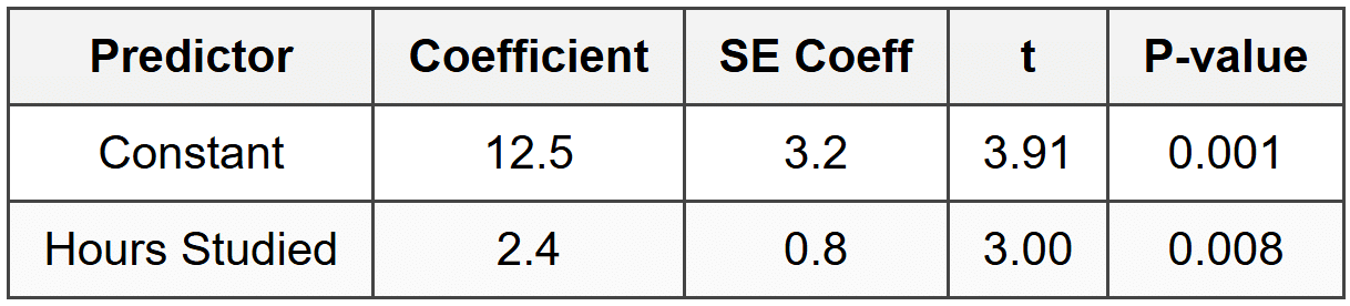
In this table:

• Constant refers to the y-intercept of the regression line.
• Hours Studied is the explanatory variable. Its coefficient (2.4) is the sample slope \( b \).
• SE Coeff is the standard error. For the slope, \( SE_b = 0.8 \).
• t is the test statistic: \( t = 2.4 / 0.8 = 3.00 \).
• P-value is 0.008, which is the two-tailed P-value for testing \( H_0: \beta = 0 \) against \( H_a: \beta \ne 0 \).

From this output, we see that the P-value is 0.008, which is less than 0.05. Therefore, we would reject the null hypothesis and conclude there is convincing evidence of a linear relationship between hours studied and exam score.

Common Misconceptions and Important Notes

When conducting inference about slope, several common errors and misunderstandings can occur. Here are key points to keep in mind:

Causation versus Association

A statistically significant slope tells us there is an association between the two variables. It does not prove that changes in the explanatory variable cause changes in the response variable. Causation can only be established through a well-designed randomized experiment. If the data come from an observational study, confounding variables might explain the relationship.

Think of it this way: if we find a significant positive relationship between ice cream sales and drowning incidents, it doesn't mean eating ice cream causes drowning. Both variables are associated with a third variable-warm weather-which is a confounding factor.

Extrapolation

The regression line and any inference we make are valid only within the range of \( x \)-values in our data. Predicting far outside this range, called extrapolation, is risky because we don't know if the linear relationship continues beyond the observed data.

Outliers and Influential Points

A single unusual data point, especially one with an extreme \( x \)-value, can have a large effect on the slope of the regression line. Such a point is called an influential point. Always examine scatterplots and residual plots to check for outliers. If an outlier is present, consider whether it should be investigated further or whether the analysis should be done with and without it to see how much it affects the results.

Conditions Must Be Checked

Never skip checking the LINE conditions. If the relationship is curved, if residuals show a pattern, or if residuals are not normal, the t-procedures may give misleading results. In such cases, a transformation of the data or a different model may be needed.

Connecting Hypothesis Tests and Confidence Intervals

There is a close connection between a two-sided hypothesis test and a confidence interval. If a 95% confidence interval for the slope does not contain zero, then a two-sided test at the \( \alpha = 0.05 \) level would reject \( H_0: \beta = 0 \). Conversely, if the confidence interval does contain zero, we would fail to reject the null hypothesis.

This connection is useful: the confidence interval not only tells us whether the relationship is statistically significant, but also gives us a range of plausible values for the slope, which provides more information than the test alone.

Practical Steps for Performing Inference About Slope

Here is a streamlined process you can follow whenever you need to perform inference about a regression slope:

1. State the parameter of interest: Identify that you're interested in \( \beta \), the true slope of the relationship in the population.
2. Check conditions: Verify the LINE conditions using plots (scatterplot for linearity, residual plot for equal variance and independence, histogram or normal plot for normality).
3. State hypotheses (for a test): Write \( H_0 \) and \( H_a \) clearly, using proper notation.
4. Calculate the test statistic or confidence interval: Use the formulas provided or read the values from computer output.
5. Find the P-value (for a test) or critical value (for an interval): Use technology or a t-table with \( df = n - 2 \).
6. Make a decision or interpret the interval: For a test, compare the P-value to \( \alpha \) and state your conclusion in context. For an interval, interpret the range of plausible slope values in context.
7. Write a conclusion in context: Always relate your statistical conclusion back to the real-world situation.

Example:  A car manufacturer wants to understand how vehicle weight (in thousands of pounds) affects fuel efficiency (in miles per gallon).
A random sample of 25 cars gives a regression line with slope \( b = -5.2 \) mpg per thousand pounds and standard error \( SE_b = 1.1 \).
The conditions for inference have been checked and are satisfied.

Perform a significance test at the \( \alpha = 0.05 \) level to determine if there is evidence that heavier cars have lower fuel efficiency.

Solution:

State the hypotheses:
\( H_0: \beta = 0 \) (no relationship between weight and fuel efficiency)
\( H_a: \beta < 0="" \)="" (heavier="" cars="" have="" lower="" fuel="">

Calculate the test statistic:
\( t = \frac{-5.2 - 0}{1.1} = \frac{-5.2}{1.1} \approx -4.73 \)

Find the degrees of freedom:
\( df = 25 - 2 = 23 \)

Using technology or a t-table, the one-tailed P-value for \( t = -4.73 \) with 23 degrees of freedom is very small, approximately 0.00005.

Since \( 0.00005 < 0.05="" \),="" we="" reject="" the="" null="">

There is very strong evidence that heavier cars have lower fuel efficiency in the population of cars.

Summary

Inference about slope allows us to move beyond simply describing the relationship in our sample data and make conclusions about the true relationship in the population. By checking the LINE conditions, calculating a test statistic or confidence interval, and interpreting the results carefully, we can determine whether two variables are truly related or whether an observed pattern could be due to random chance. Remember that statistical significance does not imply causation and that results should always be interpreted in the context of the data and the research question. With careful application of these methods, we gain powerful tools for understanding relationships between variables in the real world.