Chapter Notes: Analysis of Variance (Anova)

Table of Contents
1. The Basic Idea Behind ANOVA
2. Assumptions of ANOVA
3. Hypotheses in ANOVA
4. The ANOVA Table and Calculations
5. Conducting an ANOVA Test
6. Interpreting ANOVA Results
7. Post-Hoc Tests
8. Effect Size in ANOVA
9. One-Way ANOVA vs. Other ANOVA Designs
10. Practical Considerations
View more

When we need to compare the averages of three or more groups, we face a challenge. Running multiple t-tests between every pair of groups increases the chance of making errors. Analysis of Variance, commonly called ANOVA, is a statistical method that allows us to test whether the means of several groups are significantly different from one another in a single, efficient test. ANOVA examines the variation within each group and compares it to the variation between the groups. If the between-group variation is much larger than the within-group variation, we have evidence that at least one group mean differs from the others.

The Basic Idea Behind ANOVA

ANOVA separates the total variation in our data into two components: variation between groups and variation within groups. Think of ANOVA like comparing different cooking classes. If students in one class consistently score much higher than students in other classes, the difference between classes is large. But if scores vary widely within each class, it's harder to say one class is truly better than another.

The core logic is straightforward:

• Between-group variation measures how much the group means differ from the overall mean. This captures the effect of the factor we are testing (such as different teaching methods or fertilizer types).
• Within-group variation measures how much individual observations differ from their own group mean. This represents random variation or natural variability within each treatment.

If the treatment really matters, the between-group variation should be substantially larger than the within-group variation. ANOVA quantifies this comparison using a test statistic called the F-statistic.

Assumptions of ANOVA

Before conducting an ANOVA test, we must verify that our data meet certain conditions. These assumptions ensure that the test results are valid and reliable.

Independence

Each observation must be independent of all other observations. This means that the value of one data point does not influence or depend on another. Independence is typically achieved through proper random sampling or random assignment to groups.

Normality

The data within each group should follow an approximate normal distribution. ANOVA is reasonably robust to violations of normality, especially when sample sizes are large and roughly equal across groups. We can check normality using histograms, normal probability plots, or statistical tests like the Shapiro-Wilk test.

Equal Variances (Homogeneity of Variance)

The population variances of all groups should be approximately equal. This assumption is called homoscedasticity. We can assess this using Levene's test or by comparing the sample standard deviations. A common rule of thumb is that the largest standard deviation should not be more than twice the smallest standard deviation.

Hypotheses in ANOVA

ANOVA tests a specific pair of hypotheses about the population means.

The null hypothesis (\(H_0\)) states that all group means are equal:

where \(k\) represents the number of groups, and \(\mu_1, \mu_2, \ldots, \mu_k\) are the population means of each group.

The alternative hypothesis (\(H_a\)) states that at least one group mean differs from the others:

Notice that the alternative hypothesis does not specify which means differ or how many differ. It simply states that not all means are equal. If we reject the null hypothesis, we know that differences exist, but we need additional analyses (called post-hoc tests) to determine exactly which groups differ.

The ANOVA Table and Calculations

ANOVA organizes calculations into a structured table that breaks down the total variation into its components. Understanding this table is essential for interpreting ANOVA results.

Partitioning the Total Sum of Squares

The total variation in the data is measured by the Total Sum of Squares (SST), which represents how much all observations vary from the grand mean (the overall mean of all data combined):

Here, \(x_{ij}\) is the \(j\)-th observation in the \(i\)-th group, and \(\bar{x}\) is the grand mean.

The total variation is divided into two parts:

The Sum of Squares Between Groups (SSB) or Treatment Sum of Squares measures variation between group means:

where \(n_i\) is the sample size of group \(i\), and \(\bar{x}_i\) is the mean of group \(i\).

The Sum of Squares Within Groups (SSW) or Error Sum of Squares measures variation within groups:

An important identity in ANOVA is that these components add up:

Degrees of Freedom

Each sum of squares has associated degrees of freedom (df):

• df for Between Groups: \(df_B = k - 1\), where \(k\) is the number of groups
• df for Within Groups: \(df_W = N - k\), where \(N\) is the total number of observations
• df for Total: \(df_T = N - 1\)

Mean Squares

To compare variances fairly, we convert sums of squares to mean squares by dividing by their respective degrees of freedom:

The Mean Square Between (MSB) estimates the variance between groups, while the Mean Square Within (MSW) estimates the variance within groups (pooled across all groups).

The F-Statistic

The test statistic for ANOVA is the F-statistic, which is the ratio of the two mean squares:

This ratio compares between-group variation to within-group variation. If the null hypothesis is true (all group means are equal), we expect \(F\) to be close to 1. If the alternative hypothesis is true, \(F\) will be substantially larger than 1 because the between-group variation will exceed what we would expect from random chance alone.

The F-statistic follows an F-distribution with \(df_B = k-1\) degrees of freedom in the numerator and \(df_W = N-k\) degrees of freedom in the denominator.

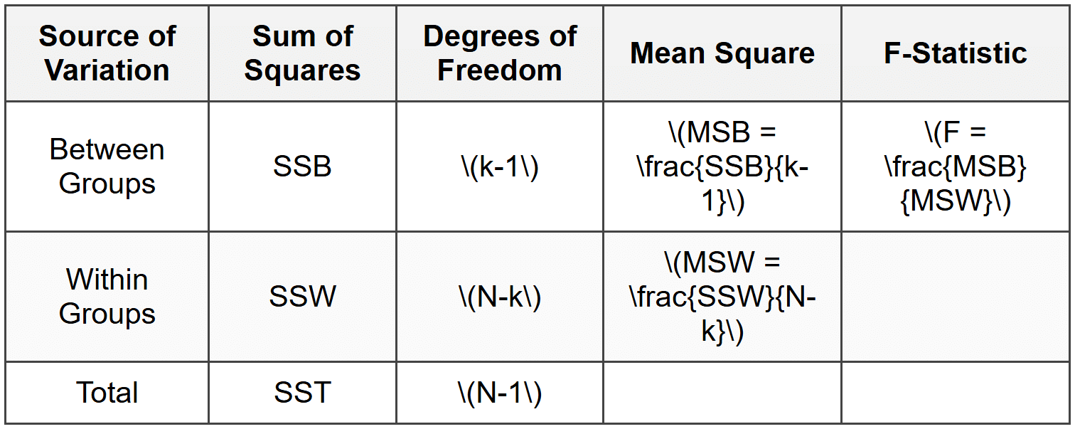
The ANOVA Table Structure

All these calculations are typically summarized in an ANOVA table:

Conducting an ANOVA Test

Let's work through a complete example to see how ANOVA works in practice.

Example:  A researcher wants to test whether three different study methods produce different exam scores.
She randomly assigns 15 students to three groups of 5 students each.
Group 1 uses flashcards, Group 2 uses practice tests, and Group 3 uses re-reading notes.

The exam scores (out of 100) are:

• Group 1 (Flashcards): 78, 82, 85, 80, 75
• Group 2 (Practice Tests): 88, 92, 85, 90, 95
• Group 3 (Re-reading): 72, 75, 70, 73, 70

Test at the \(\alpha = 0.05\) significance level whether the mean scores differ among the three study methods.

Solution:

Step 1: State the hypotheses
\(H_0: \mu_1 = \mu_2 = \mu_3\) (all three study methods produce equal mean scores)
\(H_a:\) At least one mean differs

Step 2: Calculate group means and the grand mean
Group 1 mean: \(\bar{x}_1 = \frac{78+82+85+80+75}{5} = \frac{400}{5} = 80\)
Group 2 mean: \(\bar{x}_2 = \frac{88+92+85+90+95}{5} = \frac{450}{5} = 90\)
Group 3 mean: \(\bar{x}_3 = \frac{72+75+70+73+70}{5} = \frac{360}{5} = 72\)
Grand mean: \(\bar{x} = \frac{400+450+360}{15} = \frac{1210}{15} = 80.67\)

Step 3: Calculate SSB (Sum of Squares Between)
\(SSB = 5(80-80.67)^2 + 5(90-80.67)^2 + 5(72-80.67)^2\)
\(SSB = 5(-0.67)^2 + 5(9.33)^2 + 5(-8.67)^2\)
\(SSB = 5(0.4489) + 5(87.0489) + 5(75.1689)\)
\(SSB = 2.2445 + 435.2445 + 375.8445 = 813.33\)

Step 4: Calculate SSW (Sum of Squares Within)
For Group 1: \((78-80)^2 + (82-80)^2 + (85-80)^2 + (80-80)^2 + (75-80)^2 = 4+4+25+0+25 = 58\)
For Group 2: \((88-90)^2 + (92-90)^2 + (85-90)^2 + (90-90)^2 + (95-90)^2 = 4+4+25+0+25 = 58\)
For Group 3: \((72-72)^2 + (75-72)^2 + (70-72)^2 + (73-72)^2 + (70-72)^2 = 0+9+4+1+4 = 18\)
\(SSW = 58 + 58 + 18 = 134\)

Step 5: Calculate degrees of freedom
\(df_B = k - 1 = 3 - 1 = 2\)
\(df_W = N - k = 15 - 3 = 12\)

Step 6: Calculate mean squares
\(MSB = \frac{813.33}{2} = 406.67\)
\(MSW = \frac{134}{12} = 11.17\)

Step 7: Calculate the F-statistic
\(F = \frac{406.67}{11.17} = 36.41\)

Step 8: Find the critical value and make a decision
Using an F-table with \(df_1 = 2\) and \(df_2 = 12\) at \(\alpha = 0.05\), the critical value is approximately 3.89.
Since \(F = 36.41 > 3.89\), we reject the null hypothesis.

We have strong evidence that the mean exam scores differ among the three study methods. The F-statistic of 36.41 is highly significant, indicating that at least one study method produces different results from the others.

Interpreting ANOVA Results

When we reject the null hypothesis in ANOVA, we conclude that at least one group mean is different from the others. However, ANOVA does not tell us which specific groups differ. The test only tells us that differences exist somewhere among the groups.

The p-value associated with the F-statistic indicates the probability of observing an F-statistic as extreme as ours (or more extreme) if the null hypothesis were true. A small p-value (typically less than 0.05) provides evidence against the null hypothesis.

In the previous example, the very large F-statistic would correspond to a very small p-value (much less than 0.001), giving us very strong evidence that the study methods produce different mean scores.

Post-Hoc Tests

After finding a significant F-statistic, we often want to know which specific pairs of groups differ. Post-hoc tests (also called multiple comparison procedures) allow us to make these pairwise comparisons while controlling the overall error rate.

Common post-hoc tests include:

Tukey's Honestly Significant Difference (HSD)

Tukey's HSD test compares all possible pairs of means while controlling the family-wise error rate. It is the most commonly used post-hoc test when sample sizes are equal or nearly equal. The test computes a minimum difference required for two means to be considered significantly different.

Bonferroni Correction

The Bonferroni method adjusts the significance level for each individual comparison. If we are making \(m\) comparisons, we use \(\alpha/m\) as the significance level for each test. This method is very conservative but simple to apply.

Scheffé's Test

Scheffé's test is the most conservative post-hoc test but allows for more complex comparisons beyond simple pairwise tests. It is appropriate when you want to compare combinations of groups or when sample sizes are very unequal.

Example:  Continuing from the previous study methods example, use Tukey's HSD to determine which specific study methods differ.
The critical value from the Studentized Range distribution with \(k=3\) and \(df_W=12\) at \(\alpha=0.05\) is approximately \(q = 3.77\).

Which pairs of study methods produce significantly different mean scores?

Solution:

Step 1: Calculate the Tukey HSD critical difference
\(HSD = q \times \sqrt{\frac{MSW}{n}}\)
\(HSD = 3.77 \times \sqrt{\frac{11.17}{5}} = 3.77 \times \sqrt{2.234} = 3.77 \times 1.495 = 5.64\)

Step 2: Calculate all pairwise differences
Difference between Group 1 and Group 2: \(|80 - 90| = 10\)
Difference between Group 1 and Group 3: \(|80 - 72| = 8\)
Difference between Group 2 and Group 3: \(|90 - 72| = 18\)

Step 3: Compare each difference to HSD
Group 1 vs. Group 2: \(10 > 5.64\) → significant difference
Group 1 vs. Group 3: \(8 > 5.64\) → significant difference
Group 2 vs. Group 3: \(18 > 5.64\) → significant difference

All three pairs of study methods produce significantly different mean scores. Practice tests (Group 2) produced the highest mean score of 90, flashcards (Group 1) produced a middle score of 80, and re-reading (Group 3) produced the lowest score of 72.

Effect Size in ANOVA

Statistical significance tells us whether differences exist, but it does not tell us how large or practically important those differences are. Effect size measures provide this additional information.

Eta-Squared (η²)

Eta-squared represents the proportion of total variance in the dependent variable that is explained by the independent variable (the grouping factor):

Values of \(\eta^2\) range from 0 to 1. Common interpretations suggest:

• Small effect: \(\eta^2 \approx 0.01\)
• Medium effect: \(\eta^2 \approx 0.06\)
• Large effect: \(\eta^2 \approx 0.14\)

Omega-Squared (ω²)

Omega-squared is a less biased estimate of effect size, especially useful for smaller samples:

For our study methods example:

This indicates that approximately 86% of the variance in exam scores is explained by the choice of study method, which represents a very large effect.

One-Way ANOVA vs. Other ANOVA Designs

The ANOVA we have discussed is called one-way ANOVA because it involves one independent variable (one factor) that divides observations into groups. However, more complex designs exist for more sophisticated research questions.

Two-Way ANOVA

Two-way ANOVA includes two independent variables (factors) and can test for main effects of each factor as well as their interaction. For example, we might study the effects of both study method and time of day (morning vs. evening) on exam scores.

Repeated Measures ANOVA

When the same subjects are measured multiple times under different conditions, we use repeated measures ANOVA. This design accounts for the correlation between measurements from the same individual.

Practical Considerations

Sample Size

ANOVA requires adequate sample size to detect meaningful differences. Larger samples increase statistical power, making it easier to detect true differences when they exist. Unequal sample sizes across groups reduce power and complicate the analysis, though ANOVA can still be performed.

Violations of Assumptions

When assumptions are violated, alternatives exist:

• For serious violations of normality, consider the Kruskal-Wallis test, a non-parametric alternative to ANOVA.
• For unequal variances, Welch's ANOVA adjusts the F-statistic and degrees of freedom to accommodate heterogeneity of variance.
• Data transformations (such as log or square root transformations) can sometimes help meet assumptions.

Practical vs. Statistical Significance

With very large samples, even tiny differences can become statistically significant. Always consider whether observed differences are large enough to matter in practical terms. Effect sizes help make this judgment.