Chapter Notes: Exponential Growth & Decay


Imagine you invest $100 and it doubles every year, or a rumor spreads through a school where each person tells two more people every hour. These situations don't grow by adding the same amount each time-they grow by multiplying by the same factor repeatedly. This type of pattern is called exponential growth. On the flip side, when a car loses half its value every few years or a medicine decreases in your bloodstream by a certain percentage each hour, we see exponential decay. Understanding exponential growth and decay helps us model real-world phenomena in science, finance, population studies, and many other fields.
What Makes Growth or Decay Exponential?
In earlier math courses, you studied linear functions where the output changes by a constant amount for each unit increase in the input. For example, if you save $20 each week, your savings grow linearly. Exponential functions are different: the output changes by a constant factor (or percentage) for each unit increase in the input.
The general form of an exponential function is:
\[ y = a \cdot b^x \]where:
- \( y \) is the output or final amount
- \( a \) is the initial value (the starting amount when \( x = 0 \))
- \( b \) is the base, representing the growth or decay factor
- \( x \) is the input, often representing time
When \( b > 1 \), the function shows exponential growth because the quantity increases over time. When \( 0 < b="">< 1="" \),="" the="" function="" shows="">exponential decay because the quantity decreases over time.
Understanding Exponential Growth
Exponential growth occurs when a quantity increases by a fixed percentage or factor over equal intervals of time. This happens in situations like population growth, compound interest, viral spread of information, and bacteria reproduction.
The Exponential Growth Model
We can write the exponential growth function as:
\[ y = a \cdot b^x \]where \( b > 1 \). Alternatively, when dealing with percentage growth rates, we often use:
\[ y = a(1 + r)^x \]In this version:
- \( a \) is the initial amount
- \( r \) is the growth rate expressed as a decimal (for example, 5% = 0.05)
- \( x \) is the number of time periods
- \( 1 + r \) is the growth factor \( b \)
The expression \( 1 + r \) represents the original amount (1) plus the additional growth (r). For instance, if something grows by 20% each year, the growth factor is \( 1 + 0.20 = 1.20 \), meaning it becomes 120% of what it was the previous year.
Example: A population of 500 rabbits increases by 15% each year.
Write an equation to model the rabbit population after \( x \) years.What is the population after 4 years?
Solution:
The initial population is \( a = 500 \).
The growth rate is \( r = 0.15 \), so the growth factor is \( b = 1 + 0.15 = 1.15 \).
The exponential growth equation is \( y = 500(1.15)^x \).
To find the population after 4 years, substitute \( x = 4 \):
\( y = 500(1.15)^4 \)
\( y = 500(1.74900625) \)
\( y ≈ 874.5 \)Since we cannot have half a rabbit, we round to the nearest whole number. The population after 4 years is approximately 875 rabbits.
Example: You invest $1,200 in an account that earns 6% interest compounded annually.
How much money will you have after 10 years?
Solution:
The initial investment is \( a = 1200 \).
The annual growth rate is \( r = 0.06 \), giving us a growth factor of \( b = 1.06 \).
The equation is \( y = 1200(1.06)^x \).
Substitute \( x = 10 \):
\( y = 1200(1.06)^{10} \)
\( y = 1200(1.790847697) \)
\( y ≈ 2149.02 \)After 10 years, you will have approximately $2,149.02.
Recognizing Exponential Growth from Tables
When you examine a table of values, exponential growth reveals itself through a consistent multiplicative pattern. Each output is multiplied by the same factor as the input increases by 1.
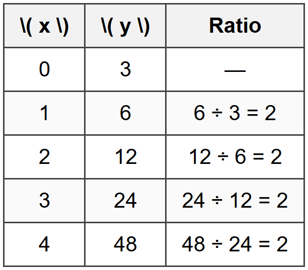
The constant ratio of 2 indicates exponential growth with \( a = 3 \) and \( b = 2 \), giving the function \( y = 3 \cdot 2^x \).
Understanding Exponential Decay
Exponential decay occurs when a quantity decreases by a fixed percentage or factor over equal intervals of time. This pattern appears in radioactive decay, depreciation of assets, cooling of hot objects, and elimination of medicine from the body.
The Exponential Decay Model
The exponential decay function has the form:
\[ y = a \cdot b^x \]where \( 0 < b="">< 1="" \).="" when="" dealing="" with="" percentage="" decay="" rates,="" we="">
\[ y = a(1 - r)^x \]In this version:
- \( a \) is the initial amount
- \( r \) is the decay rate expressed as a decimal (for example, 25% = 0.25)
- \( x \) is the number of time periods
- \( 1 - r \) is the decay factor \( b \)
The expression \( 1 - r \) represents what remains after the decay. For instance, if something loses 30% of its value each year, it retains 70%, so the decay factor is \( 1 - 0.30 = 0.70 \).
Example: A car purchased for $28,000 depreciates at a rate of 12% per year.
What is the car's value after 5 years?
Solution:
The initial value is \( a = 28000 \).
The decay rate is \( r = 0.12 \), so the decay factor is \( b = 1 - 0.12 = 0.88 \).
The exponential decay equation is \( y = 28000(0.88)^x \).
Substitute \( x = 5 \):
\( y = 28000(0.88)^5 \)
\( y = 28000(0.5277319168) \)
\( y ≈ 14776.49 \)After 5 years, the car's value is approximately $14,776.49.
Example: A medication has a half-life of 4 hours, meaning half of the medicine is eliminated from the bloodstream every 4 hours.
If a patient takes a 200 mg dose, how much remains after 12 hours?Solution:
The initial amount is \( a = 200 \) mg.
Since the medication has a half-life of 4 hours, every 4 hours the amount is multiplied by \( \frac{1}{2} = 0.5 \).
After 12 hours, there are \( 12 \div 4 = 3 \) half-life periods.
The amount remaining is:
\( y = 200(0.5)^3 \)
\( y = 200(0.125) \)
\( y = 25 \)After 12 hours, 25 mg of medication remains in the bloodstream.
Recognizing Exponential Decay from Tables
In a table showing exponential decay, each output value is multiplied by the same constant factor (less than 1) as the input increases by 1.
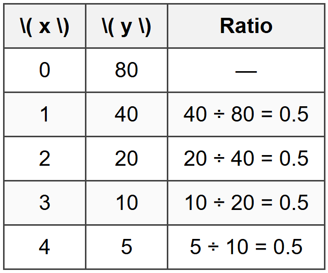
The constant ratio of 0.5 indicates exponential decay with \( a = 80 \) and \( b = 0.5 \), giving the function \( y = 80(0.5)^x \).
Comparing Exponential and Linear Functions
It's important to distinguish between linear and exponential relationships because they behave very differently, especially over longer time periods.
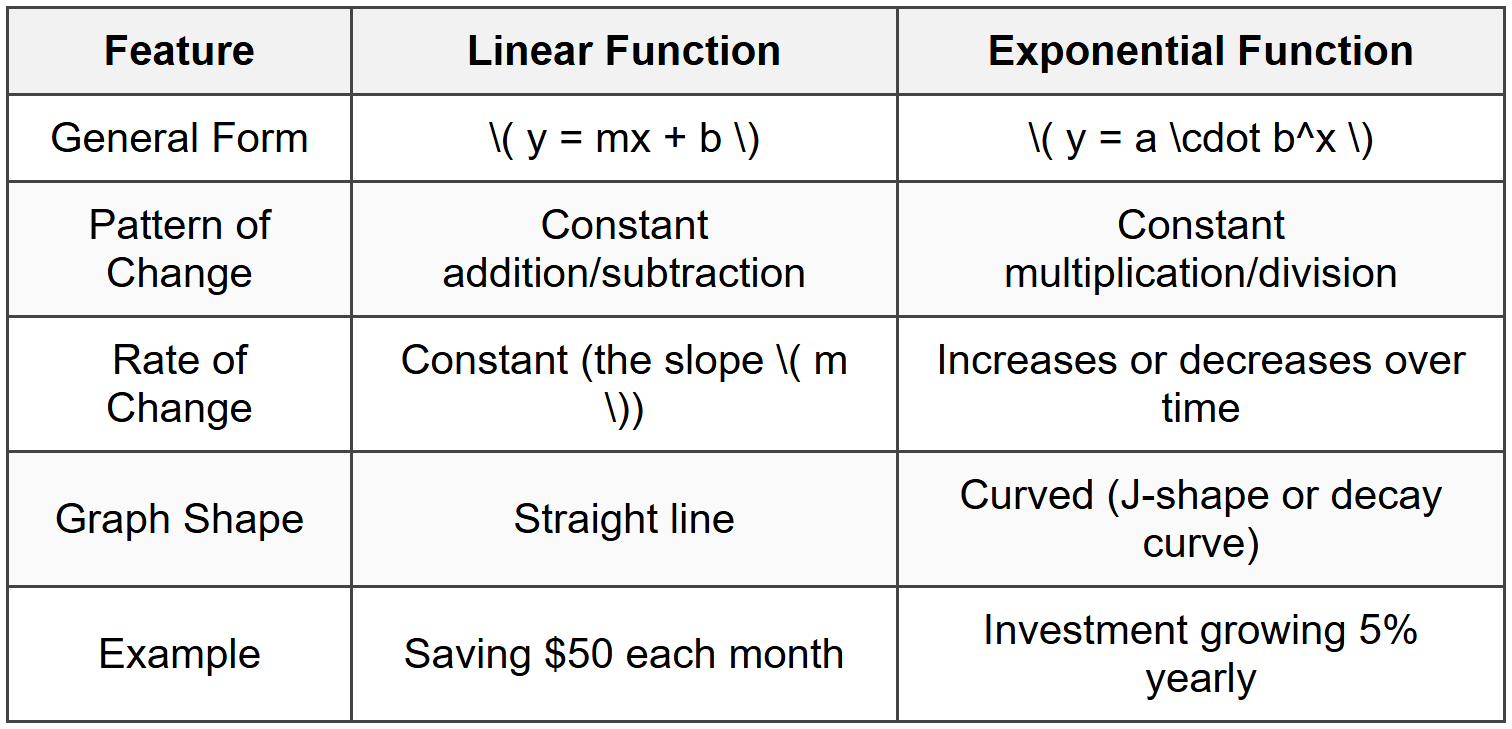
In the short term, linear and exponential functions may appear similar. However, exponential functions eventually grow much faster (or decay much faster) than linear functions. Think of exponential growth like a snowball rolling down a hill-it starts small but accelerates dramatically, while linear growth is like climbing stairs at a steady pace.
Writing Exponential Functions from Information
To write an exponential function, you need to identify two key pieces of information:
- The initial value \( a \) (the amount when \( x = 0 \))
- The growth or decay factor \( b \) (or the percentage rate \( r \))
From a Percentage Rate
When given a percentage increase or decrease:
- For growth: \( b = 1 + r \) where \( r \) is the decimal form of the percentage
- For decay: \( b = 1 - r \) where \( r \) is the decimal form of the percentage
Example: A city's population is currently 45,000 and is growing at a rate of 3.5% per year.
Write an equation to model the population after \( x \) years.
Solution:
The initial population is \( a = 45000 \).
The growth rate is \( r = 0.035 \), so the growth factor is \( b = 1 + 0.035 = 1.035 \).
The exponential growth equation is \( y = 45000(1.035)^x \).
The equation modeling the city's population after \( x \) years is \( y = 45000(1.035)^x \).
From Two Points
If you know two points on an exponential function, you can find both \( a \) and \( b \). If one point has \( x = 0 \), that immediately gives you \( a \). Then use the other point to solve for \( b \).
Example: An exponential function passes through the points (0, 12) and (3, 96).
Find the equation of the function.
Solution:
Since the point (0, 12) tells us that when \( x = 0 \), \( y = 12 \), we know \( a = 12 \).
The general form is \( y = 12 \cdot b^x \).
Substitute the point (3, 96):
\( 96 = 12 \cdot b^3 \)
\( 8 = b^3 \)
\( b = 2 \)The equation is \( y = 12 \cdot 2^x \).
Graphing Exponential Functions
The graphs of exponential functions have distinctive shapes that help us recognize them visually.
Characteristics of Exponential Growth Graphs
For \( y = a \cdot b^x \) where \( a > 0 \) and \( b > 1 \):
- The graph passes through the point (0, \( a \))
- The graph curves upward, increasing more rapidly as \( x \) increases
- The graph approaches the \( x \)-axis as \( x \) becomes very negative but never touches it (the \( x \)-axis is a horizontal asymptote)
- The \( y \)-values are always positive
- The graph is always increasing from left to right
Characteristics of Exponential Decay Graphs
For \( y = a \cdot b^x \) where \( a > 0 \) and \( 0 < b="">< 1="">
- The graph passes through the point (0, \( a \))
- The graph curves downward, decreasing more slowly as \( x \) increases
- The graph approaches the \( x \)-axis as \( x \) becomes very positive but never touches it (the \( x \)-axis is a horizontal asymptote)
- The \( y \)-values are always positive
- The graph is always decreasing from left to right
A horizontal asymptote is a horizontal line that the graph approaches but never actually reaches. For the basic exponential functions we're studying, this asymptote is the line \( y = 0 \) (the \( x \)-axis).
Applications of Exponential Growth and Decay
Compound Interest
When money earns interest and that interest is added to the principal (original amount), future interest is calculated on the new total. This is called compound interest, and it follows an exponential growth pattern.
The formula for compound interest is:
\[ A = P(1 + r)^t \]where:
- \( A \) is the final amount
- \( P \) is the principal (initial amount)
- \( r \) is the annual interest rate as a decimal
- \( t \) is the time in years
Population Growth
Populations of organisms often grow exponentially when resources are abundant. Bacteria, in particular, can double in number at regular intervals.
Example: A bacteria culture starts with 250 bacteria and doubles every 3 hours.
How many bacteria will there be after 15 hours?
Solution:
The initial population is \( a = 250 \).
The bacteria double every 3 hours, so the growth factor per 3-hour period is \( b = 2 \).
After 15 hours, there are \( 15 \div 3 = 5 \) doubling periods.
The population after 15 hours is:
\( y = 250 \cdot 2^5 \)
\( y = 250 \cdot 32 \)
\( y = 8000 \)After 15 hours, there will be 8,000 bacteria.
Radioactive Decay and Half-Life
Radioactive substances decay exponentially. The half-life is the time it takes for half of the substance to decay. After one half-life, 50% remains; after two half-lives, 25% remains; after three half-lives, 12.5% remains, and so on.
Depreciation
Many assets, especially vehicles and technology, lose value over time. When this loss happens at a constant percentage rate, the value follows an exponential decay model.
Common Mistakes to Avoid
When working with exponential functions, students often make these errors:
- Confusing growth factor with growth rate: Remember that the growth factor \( b = 1 + r \), not just \( r \). A 25% increase means multiply by 1.25, not 0.25.
- Using the wrong factor for decay: A 40% decrease means you keep 60%, so multiply by 0.60, which equals \( 1 - 0.40 \).
- Mixing up \( a \) and \( b \): The initial value \( a \) is the starting amount. The base \( b \) is what you multiply by repeatedly.
- Forgetting to convert percentages to decimals: Always convert percentages before calculating. For example, 8% becomes 0.08.
- Assuming linear growth when it's exponential: Check whether the situation involves adding the same amount each time (linear) or multiplying by the same factor (exponential).
Key Formulas Summary
Here are the essential formulas for exponential growth and decay:
General Exponential Function:
\[ y = a \cdot b^x \]Exponential Growth (with percentage rate):
\[ y = a(1 + r)^x \]where \( r \) is the growth rate and \( b = 1 + r > 1 \)
Exponential Decay (with percentage rate):
\[ y = a(1 - r)^x \]where \( r \) is the decay rate and \( b = 1 - r \), with \( 0 < b="">< 1="">
Half-Life Formula:
\[ y = a \left(\frac{1}{2}\right)^{\frac{x}{h}} \]where \( h \) is the half-life period and \( x \) is the total time elapsed
Understanding exponential growth and decay gives you powerful tools to model and predict real-world situations. Whether you're calculating investment returns, predicting population changes, or understanding how quickly a new trend might spread, exponential functions provide the mathematical framework to make sense of rapid change.


