Chapter Notes: Polynomial Graphs


Polynomial functions create distinctive curves when we graph them on the coordinate plane. Understanding these curves helps us solve real-world problems involving projectile motion, business profit models, and engineering designs. In this chapter, we will explore how the degree and coefficients of a polynomial determine the shape, direction, and key features of its graph. By the end, you will be able to sketch polynomial graphs accurately and interpret what they tell us about the behavior of the function.
Understanding Polynomial Functions
A polynomial function is a function that can be written in the form:
\[ f(x) = a_n x^n + a_{n-1} x^{n-1} + \cdots + a_2 x^2 + a_1 x + a_0 \]where \( n \) is a non-negative integer called the degree of the polynomial, and \( a_n, a_{n-1, \ldots, a_0 \) are real numbers called coefficients. The coefficient \( a_n \) (the coefficient of the highest power term) is called the leading coefficient, and it cannot be zero.
The degree tells us the highest power of \( x \) in the polynomial. For example, \( f(x) = 3x^4 - 2x^2 + 5 \) has degree 4, and \( g(x) = -x^3 + 7x - 1 \) has degree 3. The degree is the most important characteristic because it determines the overall shape and behavior of the graph.
End Behavior of Polynomial Graphs
The end behavior of a polynomial describes what happens to the \( y \)-values as \( x \) approaches positive infinity (\( x \to \infty \)) or negative infinity (\( x \to -\infty \)). This behavior depends on two factors: the degree of the polynomial and the sign of the leading coefficient.
Even-Degree Polynomials
When a polynomial has an even degree (like 2, 4, 6, etc.), both ends of the graph go in the same direction:
- If the leading coefficient is positive, both ends rise upward. As \( x \to \infty \), \( f(x) \to \infty \), and as \( x \to -\infty \), \( f(x) \to \infty \).
- If the leading coefficient is negative, both ends fall downward. As \( x \to \infty \), \( f(x) \to -\infty \), and as \( x \to -\infty \), \( f(x) \to -\infty \).
Think of even-degree polynomials as having symmetric end behavior, like a parabola or a flattened version of one.
Odd-Degree Polynomials
When a polynomial has an odd degree (like 1, 3, 5, etc.), the ends of the graph go in opposite directions:
- If the leading coefficient is positive, the left end falls and the right end rises. As \( x \to \infty \), \( f(x) \to \infty \), and as \( x \to -\infty \), \( f(x) \to -\infty \).
- If the leading coefficient is negative, the left end rises and the right end falls. As \( x \to \infty \), \( f(x) \to -\infty \), and as \( x \to -\infty \), \( f(x) \to \infty \).
Odd-degree polynomials behave like elongated S-curves, with opposite ends heading in opposite directions.
Example: Determine the end behavior of \( f(x) = -2x^5 + 3x^3 - x + 4 \).
What is the end behavior of this polynomial?
Solution:
First, identify the degree: The highest power of \( x \) is 5, so the degree is 5 (odd).
Next, identify the leading coefficient: The coefficient of \( x^5 \) is -2 (negative).
Since the degree is odd and the leading coefficient is negative, the left end rises and the right end falls.
As \( x \to -\infty \), \( f(x) \to \infty \), and as \( x \to \infty \), \( f(x) \to -\infty \).
The graph rises on the left side and falls on the right side as we move away from the origin.
Zeros and x-Intercepts
The zeros (or roots) of a polynomial function are the values of \( x \) where \( f(x) = 0 \). Graphically, these are the x-intercepts, the points where the graph crosses or touches the x-axis. Finding zeros is essential because they help us sketch the graph and understand where the function changes sign.
A polynomial of degree \( n \) has at most \( n \) real zeros. These zeros can be found by factoring the polynomial or using other algebraic techniques.
Multiplicity of Zeros
The multiplicity of a zero is the number of times that zero appears as a factor. Multiplicity affects the behavior of the graph at the x-intercept:
- Odd multiplicity (1, 3, 5, ...): The graph crosses the x-axis at this zero. The function changes sign.
- Even multiplicity (2, 4, 6, ...): The graph touches the x-axis at this zero but does not cross. The function does not change sign; it bounces off the axis.
Example: Analyze the zeros and their multiplicities for \( f(x) = (x + 2)(x - 1)^2(x - 3) \).
What are the zeros, their multiplicities, and how does the graph behave at each?
Solution:
Set each factor equal to zero to find the zeros:
\( x + 2 = 0 \) gives \( x = -2 \) with multiplicity 1 (odd), so the graph crosses the x-axis at \( x = -2 \).
\( x - 1 = 0 \) gives \( x = 1 \) with multiplicity 2 (even), so the graph touches the x-axis at \( x = 1 \) and bounces back.
\( x - 3 = 0 \) gives \( x = 3 \) with multiplicity 1 (odd), so the graph crosses the x-axis at \( x = 3 \).
The zeros are -2, 1, and 3, with the graph crossing at -2 and 3, and touching at 1.
Turning Points
A turning point is a point on the graph where the function changes from increasing to decreasing, or from decreasing to increasing. These are the peaks (local maxima) and valleys (local minima) of the graph.
A polynomial of degree \( n \) has at most \( n - 1 \) turning points. For example, a cubic polynomial (degree 3) has at most 2 turning points, and a quartic polynomial (degree 4) has at most 3 turning points.
Think of turning points as the places where the graph changes direction, like the top of a hill or the bottom of a valley on a roller coaster.
Graphing Polynomial Functions Step by Step
To sketch the graph of a polynomial function accurately, follow these systematic steps:
- Determine the degree and leading coefficient to predict end behavior.
- Find all zeros by factoring or using other methods, and determine their multiplicities.
- Find the y-intercept by evaluating \( f(0) \).
- Identify the maximum number of turning points (degree minus 1).
- Plot the zeros and y-intercept on the coordinate plane.
- Sketch the curve connecting the points, making sure the graph crosses or touches at each zero according to multiplicity, and follows the correct end behavior.
Example: Sketch the graph of \( f(x) = x^3 - 4x \).
How do we graph this polynomial step by step?
Solution:
Step 1: The degree is 3 (odd) and the leading coefficient is 1 (positive), so the left end falls and the right end rises.
Step 2: Factor to find zeros: \( f(x) = x(x^2 - 4) = x(x - 2)(x + 2) \). The zeros are \( x = 0, 2, -2 \), all with multiplicity 1, so the graph crosses at each.
Step 3: The y-intercept is \( f(0) = 0 \), so the graph passes through the origin.
Step 4: Maximum turning points = \( 3 - 1 = 2 \).
Step 5: Plot the points \( (-2, 0) \), \( (0, 0) \), and \( (2, 0) \).
Step 6: The graph enters from the bottom left, crosses at \( x = -2 \), rises to a peak, falls through \( x = 0 \), drops to a valley, then crosses at \( x = 2 \) and rises to the top right.
The graph is an S-shaped curve crossing the x-axis at -2, 0, and 2, with two turning points.
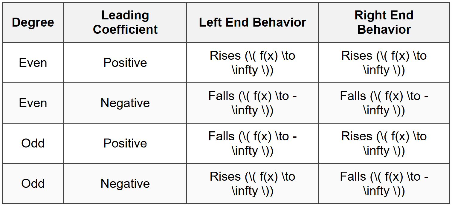
The Leading Coefficient Test
The Leading Coefficient Test is a quick method to determine end behavior without graphing the entire function. It relies solely on the degree and the sign of the leading coefficient, as summarized in this table:
Intermediate Value Theorem and Polynomial Graphs
The Intermediate Value Theorem states that if a polynomial function \( f \) is continuous on an interval \([a, b]\) and \( N \) is any number between \( f(a) \) and \( f(b) \), then there exists at least one number \( c \) in \([a, b]\) such that \( f(c) = N \).
Since polynomial functions are continuous everywhere, this theorem guarantees that if the function changes sign over an interval, there must be at least one zero in that interval. This is particularly useful for locating zeros when exact factoring is difficult.
Example: Show that \( f(x) = x^3 - x - 1 \) has a zero between \( x = 1 \) and \( x = 2 \).
How can we use the Intermediate Value Theorem?
Solution:
Evaluate \( f(1) = 1^3 - 1 - 1 = -1 \), which is negative.
Evaluate \( f(2) = 2^3 - 2 - 1 = 5 \), which is positive.
Since \( f(1) = -1 < 0="" \)="" and="" \(="" f(2)="5"> 0 \), the function changes sign on the interval \([1, 2]\).
By the Intermediate Value Theorem, there must be at least one value \( c \) in \([1, 2]\) where \( f(c) = 0 \).
Therefore, the function has at least one zero between 1 and 2.
Graphing Higher-Degree Polynomials
As the degree of a polynomial increases, the graph can have more zeros and more turning points, making the shape more complex. However, the same principles apply:
- Identify degree and leading coefficient for end behavior.
- Find all zeros and their multiplicities.
- Determine possible turning points.
- Use additional test points between zeros if needed to refine the shape.
For polynomials of degree 4 and higher, the graph may have multiple peaks and valleys. Testing points between zeros helps us understand where the graph rises and falls.
Example: Describe the graph of \( f(x) = -x^4 + 4x^2 \).
What are the key features of this graph?
Solution:
The degree is 4 (even) and the leading coefficient is -1 (negative), so both ends fall downward.
Factor: \( f(x) = -x^2(x^2 - 4) = -x^2(x - 2)(x + 2) \). The zeros are \( x = 0 \) (multiplicity 2), \( x = 2 \) (multiplicity 1), and \( x = -2 \) (multiplicity 1).
At \( x = 0 \), the graph touches the x-axis (even multiplicity). At \( x = \pm 2 \), the graph crosses the x-axis (odd multiplicity).
The maximum number of turning points is \( 4 - 1 = 3 \).
The y-intercept is \( f(0) = 0 \).
The graph enters from the bottom, crosses at \( x = -2 \), rises to a peak, touches at \( x = 0 \), rises again to another peak, crosses at \( x = 2 \), and then falls to the bottom.
The graph is a W-shaped curve with zeros at -2, 0, and 2, touching at the origin.
Symmetry in Polynomial Graphs
Some polynomial graphs have special symmetry properties that make them easier to sketch and analyze.
Even Functions
A polynomial function is an even function if \( f(-x) = f(x) \) for all \( x \). Even functions have y-axis symmetry, meaning the graph is symmetric about the y-axis. A polynomial is even if it contains only even powers of \( x \).
Example: \( f(x) = x^4 - 3x^2 + 2 \) is even.
Odd Functions
A polynomial function is an odd function if \( f(-x) = -f(x) \) for all \( x \). Odd functions have origin symmetry, meaning if you rotate the graph 180° about the origin, it looks the same. A polynomial is odd if it contains only odd powers of \( x \).
Example: \( f(x) = x^5 - 2x^3 + x \) is odd.
Recognizing symmetry reduces the work needed to sketch a graph because you only need to plot half of it and then reflect or rotate.
Summary of Key Features
When analyzing and sketching polynomial graphs, always consider these essential features:
- Degree: Determines the maximum number of zeros and turning points, and influences overall shape.
- Leading coefficient: Determines the direction of end behavior.
- Zeros and multiplicity: Determine x-intercepts and whether the graph crosses or touches at each.
- Y-intercept: Found by evaluating \( f(0) \).
- Turning points: At most \( n - 1 \) for a polynomial of degree \( n \).
- End behavior: Predicted by the Leading Coefficient Test.
- Symmetry: Identified by checking if the function is even or odd.
Mastering these features allows you to sketch accurate graphs of polynomial functions and understand their behavior across the entire domain. Whether modeling the path of a rocket, analyzing business revenue over time, or studying natural phenomena, polynomial graphs provide a powerful visual tool for interpreting mathematical relationships.


