Chapter Notes: Modeling

Table of Contents
1. Understanding Mathematical Models
2. The Modeling Cycle
3. Linear Models
4. Exponential Models
5. Quadratic Models
6. Choosing Appropriate Models
7. Interpreting Models in Context
8. Using Models to Make Predictions and Decisions
9. Limitations and Validity of Models
View more

Mathematical modeling is the process of using mathematics to represent, analyze, and solve real-world problems. When you create a mathematical model, you translate a situation from the real world into mathematical language-equations, functions, graphs, or formulas-so you can use mathematical tools to understand the situation better and make predictions. Models help scientists predict weather patterns, engineers design bridges, economists forecast market trends, and doctors plan treatment schedules. In this chapter, you will learn how to build models from data and situations, interpret what those models mean in context, and use them to answer practical questions.

Understanding Mathematical Models

A mathematical model is a mathematical representation of a real-world situation. Models are simplifications-they capture the most important features of a situation while ignoring less important details. Think of a model like a map: a map doesn't show every blade of grass or every pebble on a road, but it shows enough detail to help you navigate from one place to another.

Mathematical models can take many forms:

• Equations that relate variables, such as \( C = 50 + 20h \) for the cost of hiring a plumber
• Functions that describe how one quantity depends on another, like \( A(t) = 100(1.05)^t \) for compound interest
• Graphs that show trends and relationships visually
• Tables that organize data systematically
• Inequalities that describe constraints or limits

Every model has variables, which are quantities that can change, and parameters, which are fixed values specific to the situation. For example, in the plumber cost equation \( C = 50 + 20h \), the variable \( h \) represents hours worked (which changes), while 50 and 20 are parameters (the fixed call-out fee and hourly rate).

The Modeling Cycle

Creating and using a mathematical model follows a cycle with several stages:

1. Identify the Problem: Clearly define what question you need to answer or what situation you need to understand.
2. Make Assumptions: Decide what factors are important and what can be ignored. State your assumptions explicitly.
3. Define Variables: Choose letters to represent the quantities that change in your situation and specify their units.
4. Build the Model: Create an equation, function, or other mathematical representation based on the relationships in the situation.
5. Solve or Analyze: Use mathematical techniques to answer questions or make predictions.
6. Interpret Results: Translate mathematical answers back into the context of the original problem.
7. Validate and Refine: Check whether the model's predictions match reality. If not, revise assumptions or improve the model.

This cycle is not always linear-you may need to go back and refine your model multiple times as you learn more about the situation.

Example:  A taxi company charges a flat fee of $3.50 plus $2.25 per mile traveled.

Create a model for the total cost of a taxi ride and use it to find the cost of a 12-mile trip.

Solution:

Step 1 - Define variables:
Let \( m \) = number of miles traveled
Let \( C \) = total cost in dollars

Step 2 - Build the model:
The total cost equals the flat fee plus the per-mile charge times the number of miles:
\( C = 3.50 + 2.25m \)

Step 3 - Use the model:
For a 12-mile trip, substitute \( m = 12 \):
\( C = 3.50 + 2.25(12) \)
\( C = 3.50 + 27 \)
\( C = 30.50 \)

The cost of a 12-mile taxi ride is $30.50.

Linear Models

Many real-world situations involve constant rates of change, which can be modeled using linear functions. A linear model has the form:

where \( m \) is the slope (rate of change) and \( b \) is the y-intercept (initial value when \( x = 0 \)). In context, the slope tells you how much the dependent variable changes for each one-unit increase in the independent variable, and the y-intercept represents the starting value.

Building Linear Models from Context

When a problem describes a situation with a constant rate, you can build a linear model by identifying:

• The initial value (what happens when the independent variable is zero)
• The rate of change (how much the dependent variable increases or decreases per unit)

Example:  A water tank contains 450 gallons of water.
Water drains from the tank at a constant rate of 15 gallons per minute.

Write a linear model for the amount of water remaining after \( t \) minutes, and determine how much water remains after 20 minutes.

Solution:

Step 1 - Define variables:
Let \( t \) = time in minutes
Let \( W \) = amount of water remaining in gallons

Step 2 - Identify initial value and rate:
Initial amount: 450 gallons (when \( t = 0 \))
Rate of change: -15 gallons per minute (negative because water is draining)

Step 3 - Build the model:
\( W = 450 - 15t \)

Step 4 - Calculate for \( t = 20 \):
\( W = 450 - 15(20) \)
\( W = 450 - 300 \)
\( W = 150 \)

After 20 minutes, 150 gallons of water remain in the tank.

Finding Linear Models from Data

When you have data points from a real-world situation, you can create a linear model by finding the equation of the line that best fits the data. If the data points lie exactly on a line, you can use any two points to find the slope and then write the equation. If the points don't line up perfectly but show a linear trend, you might estimate a line of best fit or use technology to find a regression line.

To find a linear model from two data points \((x_1, y_1)\) and \((x_2, y_2)\):

1. Calculate the slope: \( m = \frac{y_2 - y_1}{x_2 - x_1} \)
2. Use point-slope form: \( y - y_1 = m(x - x_1) \)
3. Convert to slope-intercept form: \( y = mx + b \)

Example:  A scientist measures the temperature of a cooling liquid at two times:
After 5 minutes, the temperature is 78°C.
After 15 minutes, the temperature is 58°C.

Assuming the temperature decreases linearly, find a model and predict the temperature after 25 minutes.

Solution:

Step 1 - Define variables and identify points:
Let \( t \) = time in minutes, \( T \) = temperature in °C
Points: \((5, 78)\) and \((15, 58)\)

Step 2 - Calculate slope:
\( m = \frac{58 - 78}{15 - 5} = \frac{-20}{10} = -2 \)
The temperature decreases 2°C per minute.

Step 3 - Write equation using point-slope form with \((5, 78)\):
\( T - 78 = -2(t - 5) \)
\( T - 78 = -2t + 10 \)
\( T = -2t + 88 \)

Step 4 - Predict temperature at \( t = 25 \):
\( T = -2(25) + 88 \)
\( T = -50 + 88 \)
\( T = 38 \)

After 25 minutes, the model predicts a temperature of 38°C.

Exponential Models

When a quantity changes by a constant percentage rather than a constant amount, the situation is best modeled with an exponential function. Exponential models have the form:

or in contexts involving growth or decay rates:

where:

• \( a \) is the initial value (the value when \( x = 0 \) or \( t = 0 \))
• \( b \) is the base or growth/decay factor
• \( r \) is the growth rate (if positive) or decay rate (if negative) expressed as a decimal
• \( t \) is time or the independent variable

If \( b > 1 \) or \( r > 0 \), the model represents exponential growth. If \( 0 < b="">< 1="" \)="" or="" \(="" r="">< 0="" \),="" the="" model="" represents="">exponential decay.

Building Exponential Models from Context

Common exponential situations include population growth, radioactive decay, compound interest, and viral spread. To build an exponential model:

1. Identify the initial value \( a \)
2. Determine the growth or decay rate \( r \) (often given as a percentage)
3. Write the model as \( y = a(1 + r)^t \) for growth or \( y = a(1 - r)^t \) for decay

Example:  A population of bacteria starts at 200 and doubles every 3 hours.

Write an exponential model for the population after \( t \) hours, and find the population after 12 hours.

Solution:

Step 1 - Define variables:
Let \( t \) = time in hours, \( P \) = population of bacteria
Initial population: \( a = 200 \)

Step 2 - Determine the growth factor:
The population doubles every 3 hours, so every 3 hours the population is multiplied by 2.
For a model in terms of \( t \) hours, we need the population after \( t \) hours.
Number of 3-hour periods in \( t \) hours: \( \frac{t}{3} \)
Model: \( P = 200 \cdot 2^{t/3} \)

Step 3 - Calculate population at \( t = 12 \):
\( P = 200 \cdot 2^{12/3} \)
\( P = 200 \cdot 2^4 \)
\( P = 200 \cdot 16 \)
\( P = 3200 \)

After 12 hours, the population is 3,200 bacteria.

Example:  A car purchased for $28,000 depreciates at a rate of 12% per year.

Write an exponential model for the car's value after \( t \) years, and find its value after 5 years.

Solution:

Step 1 - Define variables:
Let \( t \) = time in years, \( V \) = value in dollars
Initial value: \( a = 28000 \)
Decay rate: \( r = 0.12 \)

Step 2 - Build the model:
Since the car depreciates (loses value), we use decay:
\( V = 28000(1 - 0.12)^t \)
\( V = 28000(0.88)^t \)

Step 3 - Calculate value at \( t = 5 \):
\( V = 28000(0.88)^5 \)
\( V = 28000(0.5277) \)
\( V ≈ 14775.36 \)

After 5 years, the car's value is approximately $14,775.

Quadratic Models

Some situations involve quantities that increase and then decrease, or decrease and then increase, creating a curved graph with a highest or lowest point. These situations are often best modeled with quadratic functions of the form:

where \( a \), \( b \), and \( c \) are constants. The graph of a quadratic function is a parabola. If \( a > 0 \), the parabola opens upward and has a minimum point. If \( a < 0="" \),="" the="" parabola="" opens="" downward="" and="" has="" a="" maximum="">

Common contexts for quadratic models include projectile motion (the path of a thrown ball), area problems, and profit maximization in business.

Projectile Motion Models

When an object is thrown or launched, its height over time follows a quadratic pattern due to gravity. The general model for the height \( h \) of a projectile at time \( t \) is:

where:

• \( h \) is height in feet
• \( t \) is time in seconds
• \( v_0 \) is the initial upward velocity in feet per second
• \( h_0 \) is the initial height in feet
• -16 represents half the acceleration due to gravity (in feet per second squared)

Example:  A ball is thrown upward from a platform 6 feet high with an initial velocity of 48 feet per second.

Write a model for the ball's height and find the maximum height it reaches.

Solution:

Step 1 - Build the model:
\( h_0 = 6 \), \( v_0 = 48 \)
\( h = -16t^2 + 48t + 6 \)

Step 2 - Find the maximum height:
The maximum occurs at the vertex. For \( y = ax^2 + bx + c \), the x-coordinate of the vertex is \( t = -\frac{b}{2a} \).
\( t = -\frac{48}{2(-16)} = -\frac{48}{-32} = 1.5 \) seconds

Step 3 - Calculate height at \( t = 1.5 \):
\( h = -16(1.5)^2 + 48(1.5) + 6 \)
\( h = -16(2.25) + 72 + 6 \)
\( h = -36 + 72 + 6 \)
\( h = 42 \)

The ball reaches a maximum height of 42 feet after 1.5 seconds.

Choosing Appropriate Models

An important modeling skill is recognizing which type of function best fits a given situation. Here are guidelines for choosing models:

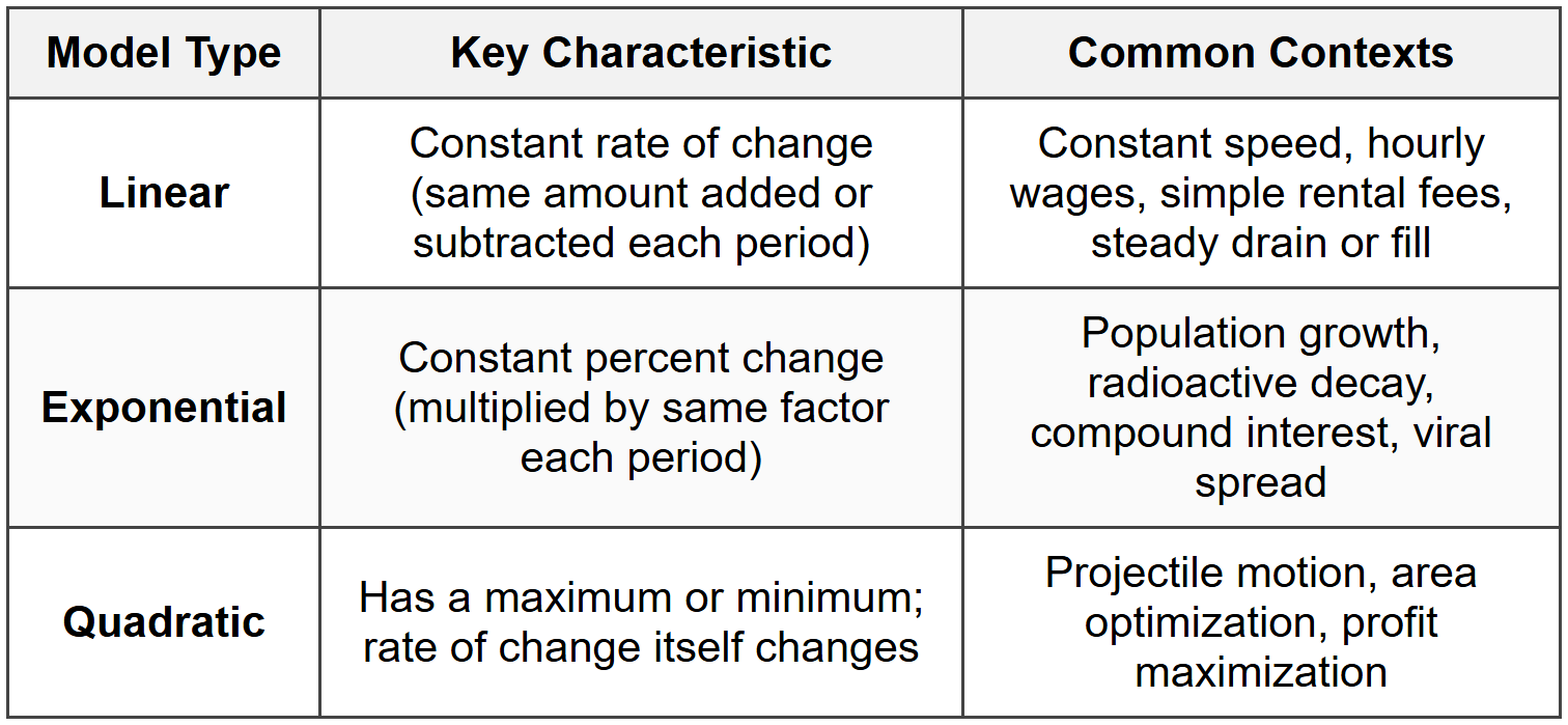
You can also use the pattern in data to identify model type:

• Linear: First differences (consecutive y-value differences) are constant
• Quadratic: Second differences are constant
• Exponential: Ratios of consecutive y-values are constant

Interpreting Models in Context

Once you have a mathematical model, it's crucial to interpret its features in terms of the real-world situation. This means translating mathematical language back into everyday language.

Interpreting Key Features

Different parts of a model have real-world meaning:

• Intercepts: The y-intercept represents the initial value or starting amount. The x-intercept(s) represent when the quantity reaches zero.
• Slope (linear models): The rate of change per unit of the independent variable.
• Maximum/Minimum (quadratic models): The highest or lowest value the quantity reaches, and when it occurs.
• Growth/Decay Factor (exponential models): How much the quantity is multiplied by each period.
• Domain restrictions: In real contexts, variables often have limits (time can't be negative, population can't be negative, etc.).

Example:  A phone plan costs $C$ dollars per month and is modeled by \( C = 45 + 0.10m \), where \( m \) is the number of minutes used beyond the included minutes.

Interpret the meaning of 45 and 0.10 in this context.

Solution:

The number 45 is the y-intercept (when \( m = 0 \)). This represents the base monthly cost of the plan when no extra minutes are used-the plan costs $45 per month for the included minutes.

The number 0.10 is the slope (rate of change). This means each additional minute beyond the included minutes costs $0.10, or 10 cents per minute.

Together, the model tells us the plan has a $45 monthly fee plus $0.10 per extra minute.

Using Models to Make Predictions and Decisions

Mathematical models are powerful tools for making predictions and informed decisions. Once you have a reliable model, you can:

• Predict future values by substituting values of the independent variable
• Determine when a certain value will be reached by solving equations
• Compare different scenarios by creating multiple models
• Optimize outcomes by finding maximum or minimum values

Solving Model Equations

Often you know the output value and need to find the input value. This requires solving an equation.

Example:  A savings account balance is modeled by \( B = 500(1.04)^t \), where \( t \) is years and \( B \) is the balance in dollars.

How many years will it take for the balance to reach $800?

Solution:

Step 1 - Set up the equation:
\( 800 = 500(1.04)^t \)

Step 2 - Isolate the exponential expression:
\( \frac{800}{500} = (1.04)^t \)
\( 1.6 = (1.04)^t \)

Step 3 - Solve using logarithms:
\( \log(1.6) = \log((1.04)^t) \)
\( \log(1.6) = t \cdot \log(1.04) \)
\( t = \frac{\log(1.6)}{\log(1.04)} \)
\( t = \frac{0.2041}{0.0170} \)
\( t ≈ 12.0 \)

It will take approximately 12 years for the balance to reach $800.

Limitations and Validity of Models

No mathematical model perfectly represents reality. Every model has limitations, and understanding these limitations is essential to using models responsibly.

Common Limitations

• Restricted domain: Models may only be valid for certain input values. For example, a population model might only work for positive time values, or a projectile model only while the object is in the air.
• Simplifying assumptions: Models ignore some factors. A projectile model might ignore air resistance; a population model might ignore migration.
• Extrapolation risks: Predicting far beyond the data you have can be unreliable. A linear model fit to data over 5 years might not accurately predict 50 years into the future.
• Changing conditions: Real-world conditions change. An exponential growth model might work while resources are unlimited, but fail when resources become scarce.

Validating Models

Always check whether a model makes sense by:

• Comparing model predictions to actual data or known outcomes
• Checking whether predicted values are reasonable in context (negative populations or heights don't make physical sense)
• Testing the model with different input values
• Considering whether the mathematical behavior matches the real-world behavior (does growth continue forever, or should it level off?)

When a model fails to match reality, you may need to refine it-choose a different function type, include additional variables, or adjust parameters based on new data. Mathematical modeling is often an iterative process where models improve through repeated testing and refinement.