NCERT Based Activity: Describing Motion Around Us

Activity 4.1: Let us analyse
- As shown in Fig. , a ball is thrown vertically upwards from O. It moves up straight till B and then falls back to O. Can this be considered a motion in a straight line?
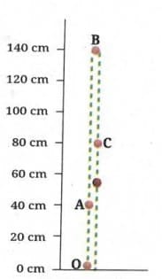 A ball in vertical motion (two separate lines are shown only for clarity; in reality, the object goes up and falls back in the same straight line)
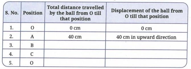
 - For this motion, fill up the values in Table .
- Analyse the data filled in Table and choose which of the following is true for displacement:
(i) It is never zero.
(ii) Its magnitude can be greater than the total distance travelled.
(iii) Its magnitude is less than or equal to the total distance travelled.
(iv) Its magnitude is less than the total distance travelled in all cases.
Observation:
Table : Distance travelled and displacement of the ball
| S. No. | Position | Total distance travelled by the ball from O till that position | Displacement of the ball from O till that position |
|---|---|---|---|
| 1. | O | 0 cm | 0 cm |
| 2. | A | 40 cm | 40 cm in upward direction |
| 3. | B | 140 cm | 140 cm in upward direction |
| 4. | C | 140 cm + (140 - 70) cm = 210 cm | 70 cm in upward direction |
| 5. | O | 280 cm | 0 cm |
(Note: From the figure, O is at 0 cm, A is at 40 cm, B is at 140 cm, C is at 70 cm on the way down. The ball travels up to B = 140 cm, then falls back. At C it has fallen 70 cm from B, so distance = 140 + 70 = 210 cm; displacement = 140 - 70 = 70 cm upward. At O again, distance = 280 cm; displacement = 0 cm.)
Answer: (iii) - Its magnitude is less than or equal to the total distance travelled.
- Yes, this can be considered motion in a straight line because the ball moves only along a vertical straight line - upward and then downward - throughout its entire journey.
- At position O (start), both distance and displacement are zero.
- As the ball moves upward, displacement equals distance since the ball moves in one direction only.
- At position B (topmost point), total distance = 140 cm and displacement = 140 cm upward; both are equal since no reversal has occurred yet.
- At position C (on the way down), total distance is greater than the magnitude of displacement, because the ball has reversed direction.
- When the ball returns to O, the total distance is 280 cm but displacement is zero, as it has returned to its starting point.
Explanation:
Distance is the total path length covered by the object, regardless of direction. It is always positive and keeps increasing. Displacement is the net change in position - it has both magnitude and direction. When the ball returns to its original position O, the displacement becomes zero even though a large distance has been covered. This shows that displacement can be zero while distance is not, and the magnitude of displacement is always less than or equal to the total distance travelled. They are equal only when the object moves in one direction without reversing.
This activity demonstrates the difference between distance and displacement, and confirms that displacement is a vector quantity while distance is a scalar quantity.
Activity 4.2: Let us calculate
- The magnitude of average acceleration of cars is generally specified as the time taken by the car to go from 0 km h⁻¹ to 100 km h⁻¹. Look it up on the internet and find this time for various cars, and record those in Table .
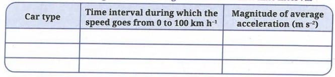
- Calculate the magnitude of average acceleration for each car.
Observation:
Table : The magnitude of average acceleration in a time interval
| Car type | Time interval during which the speed goes from 0 to 100 km h⁻¹ | Magnitude of average acceleration (m s⁻²) |
|---|---|---|
| Maruti Suzuki Swift | 13.5 s | 2.06 m s⁻² |
| Hyundai Creta | 10.8 s | 2.57 m s⁻² |
| Toyota Fortuner | 10.2 s | 2.72 m s⁻² |
| Tata Nexon EV | 8.9 s | 3.12 m s⁻² |
(Note: 100 km h⁻¹ = 27.78 m s⁻¹. Magnitude of average acceleration = 27.78 ÷ time in seconds. Values above are representative/approximate based on published data.)
- The time taken for different cars to accelerate from 0 to 100 km h⁻¹ varies considerably - ranging from about 8 to 14 seconds for typical passenger cars.
- Cars that take less time to reach 100 km h⁻¹ have a higher magnitude of average acceleration.
- Sports cars and electric vehicles generally show higher average acceleration than regular passenger cars.
- The magnitude of average acceleration is calculated as: a = (100 km h⁻¹ - 0) ÷ time interval = 27.78 m s⁻¹ ÷ t seconds.
Explanation:
Average acceleration is defined as the change in velocity divided by the time interval over which the change occurs. Mathematically:
average acceleration = (final velocity - initial velocity) ÷ time interval
Since the initial velocity is 0 and the final velocity is 100 km h⁻¹ = 27.78 m s⁻¹, the magnitude of average acceleration = 27.78 ÷ t m s⁻². A car with a smaller time t has a greater average acceleration. The SI unit of average acceleration is m s⁻². This activity demonstrates how the concept of average acceleration is applied to real-world data from cars.
Activity 4.3: Let us plot a graph
 Table : Positions of vehicle at different instants of time
- Take a sheet of graph paper. This paper is pre-divided into small squares (Fig. a), making it easier to plot data accurately.
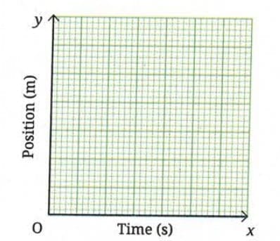 Fig.(a): Marking origin, x and y axes on graph paper
 - On the graph paper, draw two lines perpendicular to each other as shown in Fig. a. Their point of intersection is known as origin O. Mark the horizontal line as OX. It is known as the x-axis. Similarly, mark the vertical line as OY. It is called the y-axis.
- Refer to Table . We need to decide which quantity (time or position) to be shown along each axis. For the data we have (Table ), we will show time along the x-axis and position along the y-axis.
- Determine a suitable scale for each quantity to represent it on the graph paper. We need to choose scales that allow us to represent the data effectively and conveniently while utilising the available space. The scale can be:
x-axis: 5 divisions = 1 s
y-axis: 5 divisions = 20 m
- Use the chosen scale to mark values for time (1 s, 2 s, ...) along the x-axis from the origin. Similarly, mark values for position (20 m, 40 m, ...) along the y-axis (Fig. b).
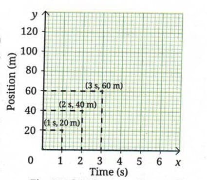 Fig.(b): Plotting points on the graph
 - Begin plotting points on the graph paper to represent each set of time and position values from Table .
(i) Table shows that at time 0 s, the position is also 0 m. The point corresponding to this set of values on the graph will therefore be the origin itself.
(ii) At 1 s, the position of vehicle is at 20 m. To mark these values, look for the point that represents 1 s on the x-axis. Draw a line parallel to the y-axis at this point. Then, draw a line parallel to the x-axis from the point corresponding to distance 20 m on the y-axis. The point where these two lines intersect represents the position 20 m at time t = 1 s on the graph (Fig.b).
(iii) Similarly, plot on the graph paper all points corresponding to positions of the vehicle at different instants of time.
- Once all points are plotted, connect them to create the position-time graph for the vehicle's motion (Fig. c). It is a straight line for the data given in Table .
 Fig.(c): Making a graph
Observation:
- All the plotted points lie exactly on a straight line passing through the origin.
- The vehicle covers equal distances (20 m) in equal time intervals (1 s) throughout its motion.
- The straight-line position-time graph indicates that the vehicle is moving with a constant velocity.
- The slope of the straight line remains the same at all points, confirming uniform motion.
Explanation:
A position-time graph represents how the position of an object changes with time. When the data points lie on a straight line, it indicates that the object is covering equal distances in equal time intervals - this is called uniform motion in a straight line, and the object has constant velocity. The slope of the position-time graph gives the magnitude of the average velocity of the object. In this case, velocity = 20 m ÷ 1 s = 20 m s⁻¹.
This activity demonstrates how to plot a position-time graph and how the shape of the graph reveals the nature of motion of an object.
Activity 4.4: Let us calculate
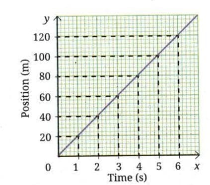 Fig.(c): Making a graph
- In the position-time graph we plotted (Fig. c), consider a part (say, AB) of the graph as shown in Fig. 1. From A, draw a line parallel to x-axis and another line parallel to Y-axis. Repeat the same from B.
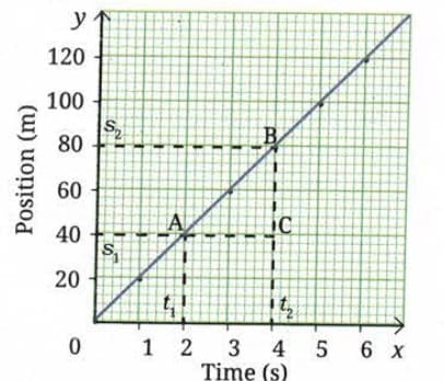 Fig.1: Calculating velocity from a position-time graph
 - Extend the horizontal line from A and a triangle ABC is formed. What do the sides BC and CA of the triangle represent? BC represents the change in position (s₂ - s₁), and AC represents the change in time (t₂ - t₁).
- As per Eq. (4.2a), by dividing the change in position (BC) by the change in time (CA), you get the average velocity:
v = (s₂ - s₁) ÷ (t₂ - t₁) = BC ÷ CA
- By extracting values of time t₁ and t₂, and distances s₁ and s₂ from the graph, the magnitude of average velocity can be calculated as:
v = (80 m - 40 m) ÷ (4 s - 2 s) = 40 m ÷ 2 s = 20 m s⁻¹
Observation:
- A triangle ABC is formed by drawing horizontal and vertical lines from points A and B on the position-time graph.
- Side BC (vertical) = change in position = s₂ - s₁ = 80 - 40 = 40 m
- Side CA (horizontal) = change in time = t₂ - t₁ = 4 - 2 = 2 s
- The ratio BC ÷ CA gives the average velocity = 20 m s⁻¹
- This value equals the slope of the straight line AB on the position-time graph.
Explanation:
The slope of a position-time graph gives the magnitude of the average velocity of the object. Geometrically, BC ÷ CA is called the slope of line AB connecting initial position A and final position B. The slope of a line is the steepness of the line - it gives the average rate of change of the quantity shown on the y-axis with respect to the quantity shown on the x-axis. Since position is on the y-axis and time is on the x-axis, the slope gives average velocity. For the straight-line graph of uniform motion, the slope is the same everywhere, confirming constant velocity = 20 m s⁻¹.
This activity demonstrates how average velocity can be determined graphically from a position-time graph using the slope of the line.
Activity 4.5: Let us investigate
- Take a ring, such as an adhesive tape ring and one marble.
- Place the ring flat on a smooth surface and throw the marble inside the ring in a way that it rotates along the inner boundary of the ring (Fig. 2).
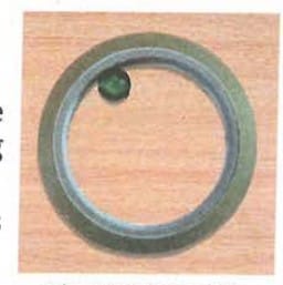 Fig.2: A marble moving inside a ring
 - Predict what will happen if you lift the ring while the marble is moving.
- Now, after one or two complete revolutions of the marble, pick up the ring without disturbing the motion of the marble. What do you observe? Does the marble continue moving in a circular motion? Or does it move in some other manner?
- Repeat the activity multiple times to confirm the result.
Observation:
- While the ring is on the surface, the marble rotates along the inner boundary of the ring in a circular path.
- When the ring is lifted, the marble does not continue in circular motion.
- Instead, the marble moves in a straight line, in the direction it was moving at the instant the ring was removed.
- Repeating the activity multiple times gives the same result - the marble always moves in a straight line after the ring is lifted.
Explanation:
When the marble moves inside the ring, the inner boundary of the ring continuously pushes the marble inward, keeping it on the circular path. This inward force from the ring is responsible for the circular motion. The moment the ring is lifted, this force is removed. Once the marble is released, it continues to move in the direction it had at that instant - which is along the tangent to the circle at the point of release. This is a straight-line path. The marble moves in a straight line because, once the ring is removed, there is no longer any force acting on it to change its direction.
This activity demonstrates that an object in circular motion moves in a straight line when released, confirming that a continuous force directed towards the centre is necessary to maintain circular motion. In uniform circular motion, although the speed is constant, the direction of velocity continuously changes - this means the object is always accelerating.
FAQs on NCERT Based Activity: Describing Motion Around Us
| 1. What is the definition of motion as discussed in the article? |  |
| 2. How can we describe the motion of an object? | |
| 3. What are the key factors that affect the motion of an object? | |
| 4. What is the significance of plotting a graph in the analysis of motion? | |
| 5. How can we calculate the speed of an object? | |


