Performance of Transmission Lines


Classification of Transmission Lines
On the basis of the length of the transmission line, transmission lines are classified into three categories:
- Short transmission lines
- Medium transmission lines
- Long transmission lines
1. Short Transmission Line
A transmission line is classed as short when its length is less than about 80 km.
Assumptions
- The shunt capacitance effect is negligible.
- The line parameters can be modelled as lumped parameters (single series impedance per phase).
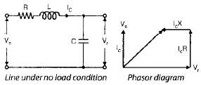
Equivalent circuit
Under balanced conditions a short transmission line is represented by a single-phase series impedance consisting of resistance R and inductive reactance XL (or series impedance Z).
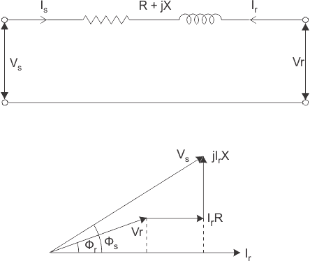
Sending-end relations
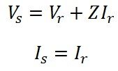
The sending-end current equals the receiving-end current under series model:
Is = Ir
The sending-end voltage is the sum of the receiving-end voltage and the voltage drop across the line impedance:
Vs = Vr + Ir Z
Voltage regulation
Voltage regulation of a line is defined as the rise in the receiving-end voltage when the full load at a specified power factor is removed while the sending-end voltage is kept constant.
% voltage regulation =
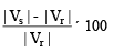
Where Vs is the sending voltage (or no-load receiving voltage) and Vr is the full-load rated receiving voltage.
From the phasor diagram of the short transmission line, the sending-end voltage can be obtained as the phasor sum of receiving voltage and impedance drop.
Where φr is the phase angle at the receiving end.
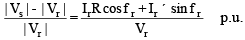
Voltage regulation =
Notes
- In the above equation φr is positive for a lagging power factor load and negative for a leading power factor load.
- The power factor strongly affects voltage regulation: for lagging power-factor loads the regulation is positive; for leading power-factor loads the regulation may be negative.
- Condition for zero voltage regulation: Ir R cos φr = Ir XL sin φr or tan φr = R / X.
Efficiency
The efficiency of the transmission line is the ratio of power at the receiving end to the power at the sending end.
% efficiency = (Power delivered at the receiving end / Power sent from the sending end) × 100
ABCD parameters (short line)
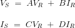
The sending-end quantities Vs, Is can be expressed in terms of the receiving-end quantities Vr, Ir by the two-port parameter form:
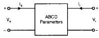
Vs = A Vr + B Ir
Is = C Vr + D Ir
- A: Voltage ratio when the receiving end is open (dimensionless).

- B: Transfer impedance; voltage at sending end to produce 1 A at short-circuited receiving end.

- C: Transfer admittance; current at sending end per volt on open-circuited receiving end.

- D: Current ratio for 1 A at short-circuited receiving end.

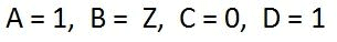
In matrix form:
- ABCD parameters of short transmission line: A = 1, B = Z, C = 0, D = 1
- Efficiency of short transmission line:

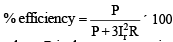
where P is the per-phase power received and R is the resistance per phase of the line.
2. Medium Transmission Line
A transmission line is classed as medium when its length lies approximately between 80 km and 240 km. The single-phase equivalent is modelled by either the nominal-T or nominal-π circuit.
Assumption
- Line parameters are still treated as lumped parameters, but shunt capacitance is no longer negligible.
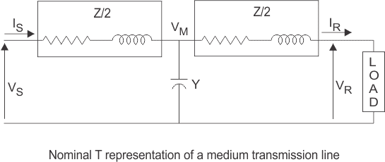
Nominal-T circuit
In the nominal-T model the shunt admittance is assumed concentrated at the midpoint and the series impedance is split into two equal halves placed on either side.
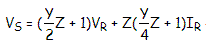
- The sending-end parameters in terms of the receiving-end parameters are derived from the T network relations.
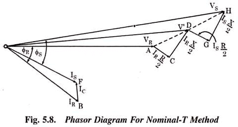
- In matrix form:
- A, B, C, D parameters for the nominal-T representation are obtained from the T-network element relationships.
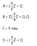
Therefore:
- Current in the shunt branch:
- Voltage across the shunt branch:

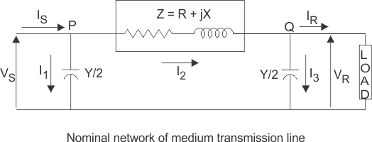
Nominal-π circuit
In the nominal-π model one half of the total line capacitance of each conductor is placed at each end; the series impedance remains in the middle.
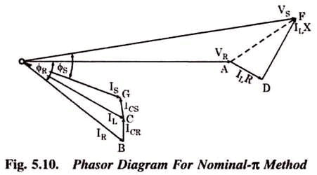
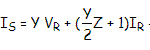
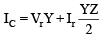
- The sending-end parameters in terms of the receiving-end parameters follow from the π network relations.
VS = A Vr + Z* Ir
- In matrix form:

- A, B, C, D parameters (for π) are obtained and are used for power flow and regulation studies.
3. Long Transmission Line
A transmission line is classed as long when its length is greater than about 240 km.
- Line parameters are distributed uniformly over the entire length (R, L, G, C per unit length).
Assumptions
- The line operates under sinusoidal, balanced, steady-state conditions.
- The line is transposed to make each phase electrically identical over the length.
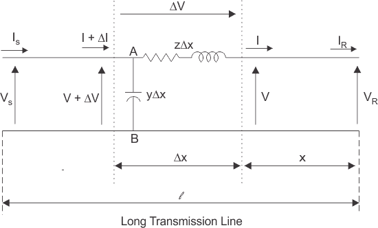
- In the figure, V(x) and I(x) denote the phasor voltage and current at distance x measured from the receiving end.
- The series impedance per unit length is z = R + jωL, where R and L are series resistance and inductance per unit length.
- The shunt admittance per unit length is y = G + jωC, where G and C are shunt conductance and capacitance to neutral per unit length.
Consider an element of infinitesimal length Δx at a distance x from the receiving end. Let:
- V = voltage just before entering the element Δx
- I = current just before entering the element Δx
- V + ΔV = voltage leaving the element Δx
- I + ΔI = current leaving the element Δx
- ΔV = voltage drop across element Δx
- z Δx = series impedance of element Δx
- y Δx = shunt admittance of element Δx
Total line impedance Z = z ℓ and total shunt admittance Y = y ℓ, where ℓ is the total line length.
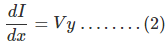
The voltage drop across the infinitesimal element Δx is given by:
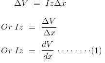
Apply Kirchhoff's current law at the node to determine ΔI:

Since the term ΔV · y · Δx is product of two infinitesimals it may be neglected; therefore:
Differentiate the equation (1) with respect to x:
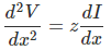
Substitute z and y relations to obtain the second-order differential equations:

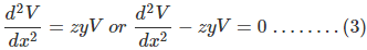
The solution of the above second-order differential equation is:

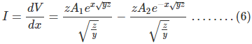
Differentiate the voltage solution with respect to x to obtain the current expression:
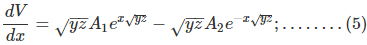
Compare with the earlier expressions to identify constants and relationships:
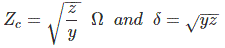
Define the characteristic impedance Zc and propagation constant γ of the long line as:
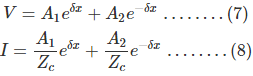
Then the voltage and current along the line can be written in terms of Zc and γ:
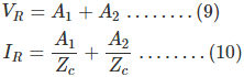
At x = 0 (receiving end) V = VR and I = IR. Substituting these conditions into the general solutions gives:
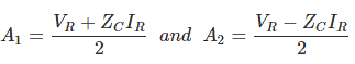
Solving for the integration constants A1 and A2 yields:
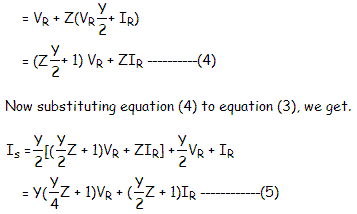
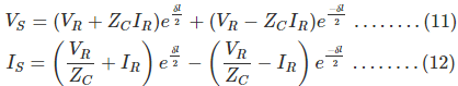
Now apply the condition at x = ℓ (sending end): V = VS, I = IS. Substituting x = ℓ and the found constants gives expressions for VS and IS:
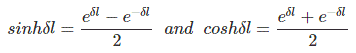
Using hyperbolic/trigonometric relations:
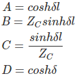
The above expressions can be re-written in compact hyperbolic form:
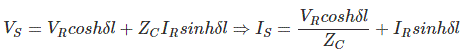
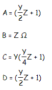
Thus, compared with the general ABCD two-port form, the ABCD parameters of a long transmission line are:
Ferranti effect
Ferranti effect: When a long line operates under no-load or very light-load conditions, the receiving-end voltage may be higher than the sending-end voltage. This phenomenon is called the Ferranti effect.
Reasons and remarks
- Usually the capacitive susceptance of the line is significant relative to its inductive susceptance for long lines; charging current causes leading reactive current in the line under light load.
- Under no-load or light load the line current is largely capacitive and leads the voltage; the capacitive charging current produces a voltage rise across the series reactance, increasing the receiving-end voltage.
- If reactive power generated at a point exceeds reactive power absorbed, the voltage at that point rises above normal and vice versa.
- Inductive reactance of the line absorbs (sinks) reactive power, while shunt capacitances generate reactive power.
- If the line loading equals the surge impedance loading (SIL), the reactive power generated by the line equals the reactive power absorbed and the voltage is uniform along the line.
- If loading is less than SIL, reactive power generated exceeds absorbed reactive power and voltages tend to rise toward the receiving end (Ferranti effect).
Power Flow On Transmission Line
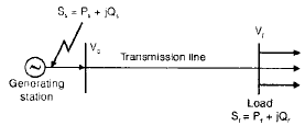
- In the typical two-bus model the sending-end bus is fed by a generator and the receiving-end supplies the load. Sr and Ss denote complex power at receiving and sending ends respectively.
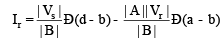
- Let receiving end voltage be Vr = |Vr| ∠0° and sending end voltage be Vs = |Vs| ∠δ. Let ABCD parameters be A = D = |A| ∠α, B = |B| ∠β.
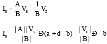
- Receiving-end current in terms of Vs, Vr and ABCD parameters:

- The complex power per phase at the receiving end:
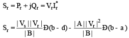
- Sending-end current in terms of Vs, Vr, and ABCD parameters:
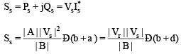
- The complex power per phase at the sending end (power injected by the generator):
Important observations
- The equations give per-phase power if phase voltages are used for Vs and Vr. Total three-phase power equals three times the per-phase power.
- If Vs and Vr are line-to-line voltages, the equations directly yield three-phase values.
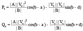
Real and reactive power expressions
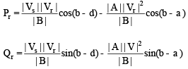
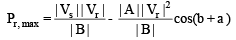
Receiving end real and reactive power expressions are:
Sending end real and reactive power expressions are:
- For fixed magnitudes |Vs| and |Vr|, the receiving end real power is maximum when the power-angle δ = β.
- The load must draw leading vars (i.e., supply negative reactive power) to achieve the condition of maximum real power transfer at the receiving end in some cases.
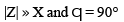
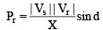
For a short transmission line, where resistance is small compared to inductive reactance:
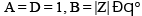
The transmission line generally has small resistance compared to reactance.

Important Conclusions
- For fixed |Vs|, |Vr| and line reactance X, the real power transferred depends on the power angle δ, which is the phase angle difference between Vs and Vr. Power can be transferred even when |Vs| = |Vr|.
- A decrease in line inductance increases the line transfer capacity.
- Inductance can be reduced by using double-circuit lines or bundled conductors, which increases transfer capability and reduces reactance-limited power transfer.
FAQs on Performance of Transmission Lines
| 1. What is the purpose of transmission lines in electrical engineering? |  |
| 2. What are the main factors that affect the performance of transmission lines? | |
| 3. How do transmission line losses affect power transmission? | |
| 4. What is the significance of impedance matching in transmission lines? | |
| 5. How does the skin effect impact the performance of transmission lines? | |


 | Explore Courses for Electrical Engineering (EE) exam |
 | Get EduRev Notes directly in your Google search |