Measurement Errors


Measurement Errors
This chapter explains the different types of errors encountered in measurements, how to quantify them, and how to estimate the maximum possible systematic error in common combinations of measured quantities. The presentation is aimed at clarity for students and practising technicians. Key terms and formulas are emphasised.
Basic Definitions
Absolute error. If the true value of a quantity is A and the measured value is Am, the absolute error is the difference between the measured value and the true value. It is written as δA and defined by
δA = Am - A
The absolute error has the same units as the measured quantity.
Relative error. The relative error is the ratio of the absolute error to the true value of the quantity. It is a dimensionless quantity, often expressed as a fraction or percentage. If the absolute error is δA, then the relative error is
εr = δA / A
Gross errors. These arise from mistakes made when reading instruments, recording values, or performing calculations. Gross errors are generally due to human mistakes and may be of any magnitude. They cannot be treated reliably by mathematical error-propagation methods and should be removed by careful checking or repeated measurement.
Systematic errors. These are reproducible, predictable deviations from the true value that remain constant or vary according to a definite law on repeated measurements. Systematic errors can usually be estimated and corrected. Two common sources are:
- Instrumental errors: inherent in the instrument due to design, calibration, wear, or mis-adjustment.
- Environmental errors: caused by operating the instrument in conditions (temperature, humidity, vibration, magnetic fields, etc.) different from those in which it was calibrated or designed.
- Environmental errors are often more troublesome because they can change with time and operating conditions.
Random (or accidental) errors. These vary in magnitude and sign in an unpredictable way and do not obey a simple law. Their presence is seen when repeated measurements of the same quantity give different results. Random errors are treated statistically (mean, standard deviation) when many measurements are available.
Determination of Maximum Systematic Error
When several measured quantities combine to give a result, each with its own possible systematic error, the maximum possible systematic error in the result can be estimated using simple rules. The rules below give the limiting (maximum) error when individual errors are independent and can act to increase or decrease the result in the worst possible way.
1. Sum of Two or More Quantities
If the result y is the sum of measured quantities u, v, z, ... each with possible systematic errors ±δu, δv, δz, ..., then the corresponding limiting error in y is
δy = ± (δu + δv + δz + ...)
2. Difference of Two Quantities
If y = u - v and the quantities have possible systematic errors ±δu and ±δv, the limiting error in y is
δy = ± (δu + δv)
3. Product of Two or More Quantities
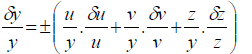
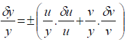
For a product y = u · v · z · ..., the maximum relative (fractional) error in y is the sum of the maximum relative errors of the factors. That is,
δy / |y| = δu / |u| + δv / |v| + δz / |z| + ...
Equivalently, the limiting absolute error is
δy = |y| (δu/|u| + δv/|v| + δz/|z| + ...)
Derivation (small-error approximation):
Assume relative changes are small and denote differentials by d.
y = u·v·z ···
d y / y = d u / u + d v / v + d z / z + ...
Replacing differentials by maximum absolute errors gives the stated relation.

4. Quotient of Two Quantities
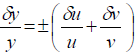
For a quotient y = u / v, the maximum relative error in y is the sum of the maximum relative errors of numerator and denominator, namely
δy / |y| = δu / |u| + δv / |v|
Thus the absolute limiting error is
δy = |y| (δu/|u| + δv/|v|)

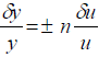
5. Power of a Single Factor
For y = un where n is any real exponent (positive, negative, integral or fractional), the maximum relative error in y is |n| times the relative error in u:
δy / |y| = |n| · (δu / |u|)
6. Composite Factor (Product of Powers)
For y = un vm, the maximum relative error is the weighted sum of relative errors:
δy / |y| = |n| · (δu / |u|) + |m| · (δv / |v|)

Resolution and Sensitivity
Resolution (or discrimination) is the smallest change in the input (the measured quantity) that an instrument can detect. Resolution may be given as an absolute value (for example, 0.01 V) or as a fraction/percentage of full-scale value (for example, 0.1% of full scale).
Sensitivity is the ratio of the output change of an instrument to a change in the input quantity. If a small change Δx in the input produces an output change Δy, the sensitivity S can be expressed as
S = Δy / Δx
High sensitivity means the instrument gives a larger output change for a small input change; however, high sensitivity alone does not guarantee good accuracy unless resolution, linearity and stability are also adequate.
Accuracy, Precision and Significant Figures
Accuracy describes the closeness between the measured value and the true value of the quantity. An instrument or a measured result is said to be accurate if the systematic errors are small or corrected.
Precision (or repeatability) refers to the closeness among repeated measurements of the same quantity under unchanged conditions. Precision is related to random errors: smaller random errors mean higher precision.
These two concepts are independent: a set of measurements can be precise but not accurate (repeatable but biased), accurate but not precise, neither, or both.
Significant figures indicate the precision of a reported numeric result. The number of significant digits retained in the final result should reflect the precision (uncertainty) of the measurement. As a rule of thumb, avoid reporting more significant figures than justified by the estimated error. For example, if a length is measured as 12.3 cm with an estimated absolute error of ±0.2 cm, reporting 12.300 cm would be misleading because the extra digits suggest a precision not supported by the error estimate.
Examples and Practical Notes
Example - Adding two measured voltages. If V1 = 10.02 V ± 0.01 V and V2 = 4.98 V ± 0.02 V, the sum V = V1 + V2 has limiting error
δV = 0.01 + 0.02 = 0.03 V
So V = 15.00 V ± 0.03 V.
Example - Multiplying current and voltage to get power. If I = 2.00 A ± 0.01 A and V = 230.0 V ± 0.5 V, then P = V·I and the relative errors add:
δP / P = δV / V + δI / I = 0.5/230.0 + 0.01/2.00
δP / P ≈ 0.002174 + 0.005 = 0.007174
So the percentage error in P is about 0.717% and the absolute error is δP = P · 0.007174.
Practical note on systematic errors. Where possible, calibrate instruments against standards, use corrections for known biases (for example, zero offsets or gain errors), and keep environmental conditions close to those used during calibration.
Practical note on random errors. Reduce random errors by averaging several independent measurements. The mean reduces random variations; the standard deviation quantifies the remaining scatter.
Understanding these basic rules and distinctions helps in planning measurements, choosing instruments, estimating uncertainty, and reporting results in a form that is both honest and useful for design, testing and decision-making.
FAQs on Measurement Errors
| 1. What are measurement errors in electrical engineering? |  |
| 2. How can instrument limitations contribute to measurement errors in electrical engineering? | |
| 3. What are some common sources of measurement errors in electrical engineering? | |
| 4. How can environmental conditions affect measurement errors in electrical engineering? | |
| 5. How can calibration help reduce measurement errors in electrical engineering? | |


 | Explore Courses for Electrical Engineering (EE) exam |
 | Get EduRev Notes directly in your Google search |