NFA to DFA Conversion

Part III. NFA to DFA Conversion
Consider the following NFA,
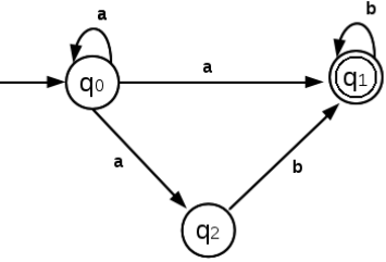
In this NFA, from state q0 there are three possible moves on the input symbol a, namely to q0, q1, and q2. When we simulate this NFA, the move from q0 on input a is non-deterministic. That means the next state is not uniquely determined by the current state and input symbol. In a deterministic finite automaton (DFA), however, for each state and each input symbol there is exactly one transition. A DFA is easier to simulate because the next state is unambiguous. For every NFA there exists an equivalent DFA that recognises the same language; the conversion procedure constructs such a DFA.
5 Epsilon Closure
Before applying the standard construction from NFA to DFA we must handle epsilon (ε) transitions. The epsilon closure (or ε-closure) of a state is central to that process.
Definition. The epsilon closure of a state q, written ECLOSE(q), is the set containing q itself and every state that can be reached from q by following zero or more ε-transitions.
To compute ECLOSE(q) one may use a depth-first or breadth-first search restricted to ε-transitions: start from q, follow all outgoing ε-transitions to new states, then continue from those states until no new states are discovered.
Example 1
Consider the following NFA.
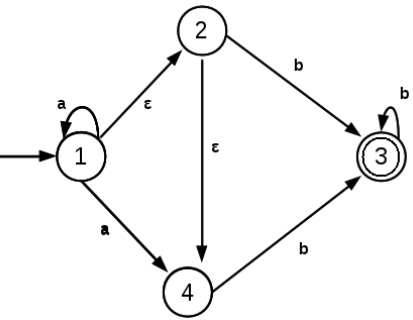
Find the epsilon closure of all states.
- ECLOSE(1) = {1, 2, 4}
- ECLOSE(2) = {2, 4}
- ECLOSE(3) = {3}
- ECLOSE(4) = {4}
Example 2
Consider the following NFA.
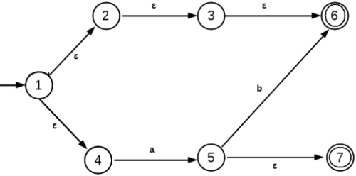
Find the epsilon closure of all states.
- ECLOSE(1) = {1, 2, 3, 6, 4}
- ECLOSE(2) = {2, 3, 6}
- ECLOSE(3) = {3, 6}
- ECLOSE(4) = {4}
- ECLOSE(5) = {5, 7}
- ECLOSE(6) = {6}
Example 3
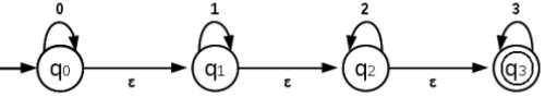
Consider the following NFA.
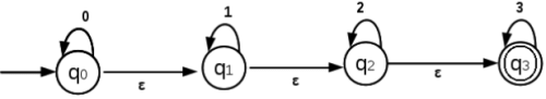
Compute the epsilon closure of all states.
- ECLOSE(q0) = {q0, q1, q2, q3}
- ECLOSE(q1) = {q1, q2, q3}
- ECLOSE(q2) = {q2, q3}
- ECLOSE(q3) = {q3}
6 Conversion of NFA to DFA
The conversion from an NFA (possibly with ε-transitions) to an equivalent DFA is performed in two main phases:
- Transform the NFA with ε-transitions to an NFA without ε-transitions (eliminate ε-transitions).
- Convert the resulting NFA (without ε-transitions) to a DFA using the subset construction (also called the powerset construction).
Both phases are described below with examples and clear step-by-step instructions.
Phase 1 - Eliminate ε-transitions
Given an NFA with ε-transitions, we construct an equivalent NFA without ε by using epsilon closures. The idea is to replace each state by its epsilon closure for transition purposes so that all ε-moves are absorbed into ordinary symbol transitions.
One systematic method:
- Compute ECLOSE(s) for every state s of the original NFA.
- For each state p and each input symbol a, compute the set of states reachable by an a-move from any state in ECLOSE(p), then take epsilon closure of that union; that is, δ'(p,a) = ECLOSE(⋃_{q in ECLOSE(p)} δ(q,a)).
- The start state of the new NFA is ECLOSE(start). Any state whose closure contains an original final state becomes final in the new NFA.
Example 1 (Eliminate ε-transitions)
Consider the NFA with ε-transitions below.
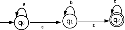
The original states are q0, q1, q2. The start state is q0. The final state is q2.
Step a: Find all epsilon closures.
- ECLOSE(q0) = {q0, q1, q2}
- ECLOSE(q1) = {q1, q2}
- ECLOSE(q2) = {q2}
The reachable sets (closures) become the states of the new NFA: {q0,q1,q2}, {q1,q2}, {q2}. The start state is {q0,q1,q2} because it is ECLOSE(start). Any of these new states that include the original final state q2 are final.
Next find transitions of these new states on input symbols a, b, c. For example, consider the composite state {q0,q1,q2} and determine where an input a, b, or c can lead by following the above algorithm.
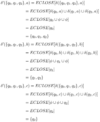
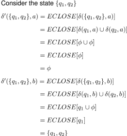
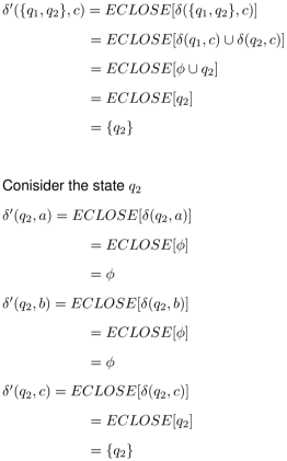
After computing these transitions we obtain the NFA without ε-transitions.
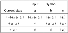
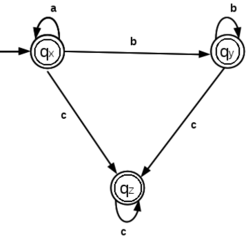
Rename the composite states for convenience:
- {q0, q1, q2} as qx
- {q1, q2} as qy
- {q2} as qz


The transition diagram of the new NFA is shown below. Note that in this particular case the resulting NFA without ε-transitions already satisfies the DFA property (one transition per symbol from each state).
Phase 2 - Subset Construction (NFA without ε to DFA)
After eliminating ε-transitions we apply the subset construction:
- The start state of the DFA is the epsilon closure of the start state of the original NFA (or simply the start state of the NFA without ε if you already removed ε).
- For each unprocessed DFA state S (S is a set of NFA states) and for each input symbol a, compute T = ⋃_{q in S} δ(q,a). If ε-transitions remain in your NFA you should take ECLOSE(T). T becomes a DFA state (possibly previously seen).
- Repeat until no new DFA state is generated.
- A DFA state S is accepting if S contains at least one accepting state of the original NFA.
Example 2 (Full conversion)
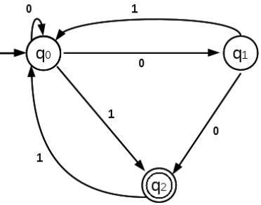
Convert the following NFA to a DFA.
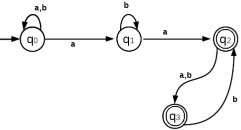
Step 1: This NFA has no ε-transitions, so we proceed directly to the subset construction.
Step a: Start with the start state q0.
- δ(q0, a) = {q0, q1}
- δ(q0, b) = {q0}
We have a new DFA state {q0, q1}.
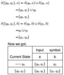
Step b: Consider {q0, q1}.
- δ({q0, q1}, a) = δ(q0, a) ∪ δ(q1, a) = {q0, q1} ∪ {q2} = {q0, q1, q2}
- δ({q0, q1}, b) = δ(q0, b) ∪ δ(q1, b) = {q0} ∪ {q1} = {q0, q1}
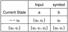
We have a new DFA state {q0, q1, q2}.
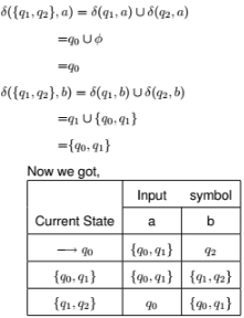
Step c: Consider {q0, q1, q2}.
- δ({q0, q1, q2}, a) = δ(q0, a) ∪ δ(q1, a) ∪ δ(q2, a) = {q0, q1} ∪ {q2} ∪ {q3} = {q0, q1, q2, q3}
- δ({q0, q1, q2}, b) = δ(q0, b) ∪ δ(q1, b) ∪ δ(q2, b) = {q0} ∪ {q1} ∪ {q3} = {q0, q1, q3}
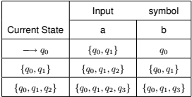
We obtain two new DFA states {q0, q1, q2, q3} and {q0, q1, q3}.
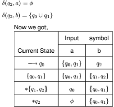
Step d: Process each of these newly generated states.
For {q0, q1, q2, q3} compute transitions (details shown below).
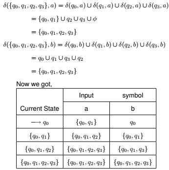
For {q0, q1, q3} compute transitions (details shown below).
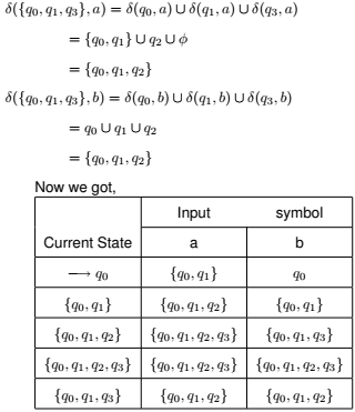
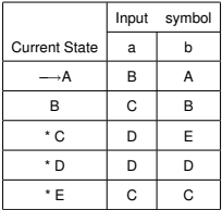
No further new states are generated. The transition table for the completed DFA is shown below. The start state is q0. DFA final states are those composite states that contain at least one final state of the original NFA (here q2 or q3).
- Final DFA states: {q0, q1, q2}, {q0, q1, q2, q3}, {q0, q1, q3}
Rename these DFA states for compactness:
- q0 as A
- {q0, q1} as B
- {q0, q1, q2} as C
- {q0, q1, q2, q3} as D
- {q0, q1, q3} as E
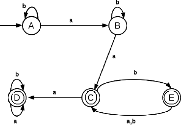
The diagram shows a DFA because from each state there is exactly one transition for each input symbol.
Example 3
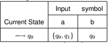
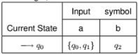
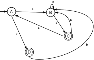
Convert the following NFA to DFA.
Step 1: This NFA contains no ε-transitions, so proceed directly to subset construction.
From the start state q0:
- δ(q0, a) = {q0, q1}
- δ(q0, b) = {q2}
Generate new composite states and compute their transitions. Intermediate tables/diagrams are shown below.
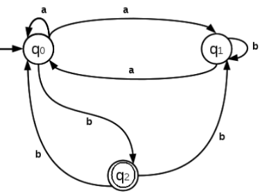
No more new states are generated. The start state is q0. Final states are q2 and {q1, q2} because they contain the original final state q2.
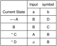
Rename composite states for convenience:
- q0 as A
- {q0, q1} as B
- {q1, q2} as C
- q2 as D
Example 4
Consider the NFA below. Convert it to a DFA.
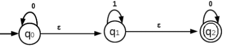
Step 1: Eliminate ε-transitions by computing closures.
- ECLOSE(q0) = {q0, q1, q2}
- ECLOSE(q1) = {q1, q2}
- ECLOSE(q2) = {q2}
The states of the new NFA are the closures above; the start state is {q0, q1, q2}. Any closure that contains the original final state q2 becomes final in the new NFA.
Now find transitions of these closures on input symbols 0 and 1. For example, consider closure {q0, q1, q2} and compute its transitions:
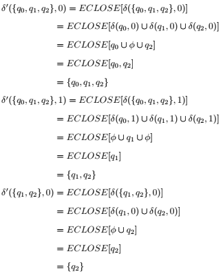
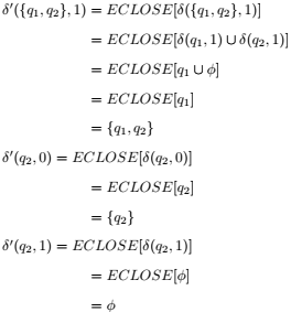
Rename closures as:
- {q0, q1, q2} as A
- {q1, q2} as B
- {q2} as C
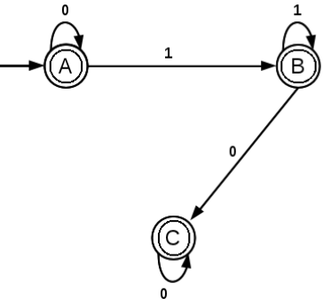
The NFA without ε-transitions shown above is already a DFA because from each state there is exactly one transition for each input symbol.
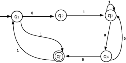
Example 5
Consider the following NFA. Convert it to a DFA.
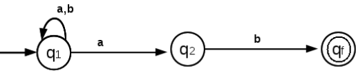
Step 1: This NFA contains no ε-transitions, so proceed to the subset construction.
Begin from the start state q1:
- δ(q1, a) = {q1, q2}
- δ(q1, b) = {q1}
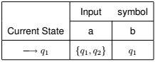
Continue computing transitions for newly generated composite states:
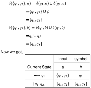
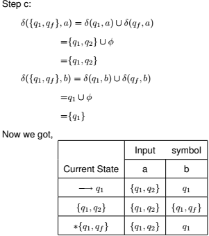
The start state is q1. The DFA accepting state is {q1, qf} because it contains the original final state qf. Rename states:
- q1 as A
- {q1, q2} as B
- {q1, qf} as C
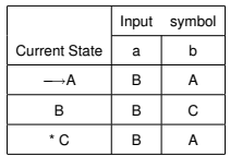
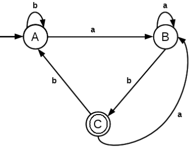
The resulting machine is a DFA because every state has exactly one transition for each input symbol.
Exercises
1. Convert the following NFA to DFA.
2. Convert the following NFA to DFA.
3. Convert the following NFA to DFA.
FAQs on NFA to DFA Conversion
| 1. What is NFA to DFA conversion in computer science engineering? |  |
| 2. Why is NFA to DFA conversion important in computer science engineering? | |
| 3. How does NFA to DFA conversion work? | |
| 4. What are the advantages of NFA to DFA conversion? | |
| 5. Are there any limitations to NFA to DFA conversion? | |


 | Explore Courses for Computer Science Engineering (CSE) exam |
 | Get EduRev Notes directly in your Google search |