Commerce Exam > Commerce Questions > Outline the steps taken in deriving saving cu...
Start Learning for Free
Outline the steps taken in deriving saving curve from the given consumption curve use diagram?
Verified Answer
Outline the steps taken in deriving saving curve from the given consum...
Deriving saving curve form consumption curve:
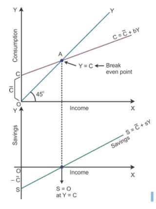
In the diagram, the consumption curve is given as C bY , where C represents the autonomous consumption, Y is income and b is the rate at which C increases corresponding to an increase in Y. The aggregate supply curve is the 45degree line. Consumption is equal to income at Point E.

Derivation of saving function from consumption function:
C is the saving function where negative savings are equal to autonomous consumption at Y = 0. This is shown on the negative axis in the lower panel at Point S. Here, all the income is spent on consumption expenditure. Hence, there is no saving which is shown as the breakeven point. After this point, S and Y are joined to have a straight line sloping curve.
 This question is part of UPSC exam. View all Commerce courses
Most Upvoted Answer
Outline the steps taken in deriving saving curve from the given consum...
Deriving the Saving Curve from the Consumption Curve
To derive the saving curve from the given consumption curve, we need to understand the relationship between consumption and saving. The saving curve represents the different levels of saving at different levels of income, while the consumption curve represents the different levels of consumption at different levels of income. Here are the steps to derive the saving curve from the consumption curve:
Step 1: Understand the Consumption Function
The consumption function shows the relationship between income and consumption. It can be expressed as C = a + bY, where C is consumption, Y is income, a is autonomous consumption (consumption when income is zero), and b is the marginal propensity to consume (the proportion of additional income that is consumed).
Step 2: Calculate Saving
Saving is the difference between income and consumption, so it can be expressed as S = Y - C. By substituting the consumption function into the saving equation, we get S = Y - (a + bY), which simplifies to S = (1 - b)Y - a. This equation represents the saving function.
Step 3: Plotting the Saving Curve
To plot the saving curve, we need to assign different levels of income and calculate the corresponding levels of saving using the saving function. The resulting data points can then be plotted on a graph with income on the x-axis and saving on the y-axis.
Step 4: Analyzing the Saving Curve
The saving curve will have a positive slope because as income increases, saving also increases. The slope of the saving curve will be equal to (1 - b), which represents the marginal propensity to save (the proportion of additional income that is saved).
Step 5: Interactions with the Consumption Curve
The saving curve intersects with the consumption curve at the equilibrium level of income, where saving equals investment. This point represents the level of income where there is no tendency for income to change. It is the point where the saving and consumption curves intersect on the graph.
Step 6: Relationship between Saving and Income
The saving curve shows the relationship between saving and income, illustrating that as income increases, saving also increases. It helps in understanding the saving behavior of individuals and the overall economy.
By following these steps, we can derive the saving curve from the given consumption curve and gain insights into the saving patterns and behavior at different levels of income.
Attention Commerce Students!
To make sure you are not studying endlessly, EduRev has designed Commerce study material, with Structured Courses, Videos, & Test Series. Plus get personalized analysis, doubt solving and improvement plans to achieve a great score in Commerce.

|
Explore Courses for Commerce exam
|

|
Similar Commerce Doubts
Outline the steps taken in deriving saving curve from the given consumption curve use diagram?
Question Description
Outline the steps taken in deriving saving curve from the given consumption curve use diagram? for Commerce 2024 is part of Commerce preparation. The Question and answers have been prepared according to the Commerce exam syllabus. Information about Outline the steps taken in deriving saving curve from the given consumption curve use diagram? covers all topics & solutions for Commerce 2024 Exam. Find important definitions, questions, meanings, examples, exercises and tests below for Outline the steps taken in deriving saving curve from the given consumption curve use diagram?.
Outline the steps taken in deriving saving curve from the given consumption curve use diagram? for Commerce 2024 is part of Commerce preparation. The Question and answers have been prepared according to the Commerce exam syllabus. Information about Outline the steps taken in deriving saving curve from the given consumption curve use diagram? covers all topics & solutions for Commerce 2024 Exam. Find important definitions, questions, meanings, examples, exercises and tests below for Outline the steps taken in deriving saving curve from the given consumption curve use diagram?.
Solutions for Outline the steps taken in deriving saving curve from the given consumption curve use diagram? in English & in Hindi are available as part of our courses for Commerce.
Download more important topics, notes, lectures and mock test series for Commerce Exam by signing up for free.
Here you can find the meaning of Outline the steps taken in deriving saving curve from the given consumption curve use diagram? defined & explained in the simplest way possible. Besides giving the explanation of
Outline the steps taken in deriving saving curve from the given consumption curve use diagram?, a detailed solution for Outline the steps taken in deriving saving curve from the given consumption curve use diagram? has been provided alongside types of Outline the steps taken in deriving saving curve from the given consumption curve use diagram? theory, EduRev gives you an
ample number of questions to practice Outline the steps taken in deriving saving curve from the given consumption curve use diagram? tests, examples and also practice Commerce tests.

|
Explore Courses for Commerce exam
|

|
Suggested Free Tests
Signup for Free!
Signup to see your scores go up within 7 days! Learn & Practice with 1000+ FREE Notes, Videos & Tests.


