Linear Inequalities Chapter Notes | Quantitative Aptitude for CA Foundation PDF Download
Chapter Overview
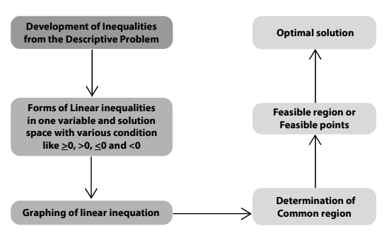
Inequalities
- Inequalities are statements indicating that two amounts are not equal, but they still have a relationship.
- These kinds of inequalities frequently appear in business when there are limits on things like supply, demand, or sales.
- For instance, if a manufacturer needs a specific type of raw material for production and there is a maximum amount available, any choices made regarding production must take this limit into account.
- This chapter will explore more examples of such situations where inequalities play a key role.
Any linear function that involves an inequality sign is a linear inequality. It may be of one variable, or, of more than one variable. Simple example of linear inequalities are those of one variable only; viz., x > 0, x ≤ 0 etc.

The values of the variables that satisfy an inequality are called the solution space, and is abbreviated as S.S. The solution spaces for
(i) x > 0,
(ii) x ≤ 0 are shaded in the above diagrams, by using deep lines.
Linear inequalities in two variables: Now we turn to linear inequalities in two variables x and y and shade a few S.S.
Let us now consider a linear inequality in two variables given by 3x + y < 6

The inequality mentioned above is true for certain pairs of numbers (x, y) that satisfy 3x + y < 6. By trial, we may arbitrarily find such a pair to be (1,1) because 3 x 1 + 1 = 4, and 4 < 6.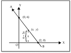
Linear inequalities in two variables may be solved easily by extending our knowledge of straight lines.
For this purpose, we replace the inequality by an equality and seek the pairs of number that satisfy 3x + y = 6.
We may write 3x + y = 6 as y = 6 – 3x, and draw the graph of this linear function.
Let x = 0 so that y = 6. Let y = 0, so that x = 2.
Any pair of numbers (x, y) that satisfies the equation y = 6 – 3x falls on the line AB.
Note: The pair of inequalities x 0, y 0 play an important role in linear programming problems.
Therefore, if y is to be less than 6 – 3x for the same value of x, it must assume a value that is less than the ordinate of length 6 – 3x.
All such points (x, y) for which the ordinate is less than 6 – 3x lie below the line AB.
- The area where these points are located is shown by an arrow and is also shaded in the diagram next to this text.
- We will look at two inequalities: 3x + y ≤ 6 and x - y ≥ -2 that both need to be true for the values of x and y.
- To find the pairs of numbers (x, y) that meet both inequalities, we can graph the lines represented by the equations y = 6 - 3x and y = 2 + x.
- After graphing, we will identify the area where both inequalities are satisfied.
- It is easier to write each equation with y on the left side and the other terms on the right side.
- The first inequality, 3x + y ≤ 6, can be rewritten as y ≤ 6 - 3x. This means that for every x, the value of y must be less than or equal to 6 - 3x.
- Therefore, the inequality is satisfied by all points that are located below the line y = 6 - 3x.
- The area where these points are found is shaded in the diagram next to this explanation.

We consider the second inequality x – y ≤ –2, and note that this is equivalent to y ≥ 2 + x. It requires the value of y for each x to be larger than or equal to that of 2 + x. The inequality is, therefore, satisfied by all points lying on and above the line y = 2 + x.
The region of interest is indicated by an arrow on the line y = 2 + x in the diagram below.
For x = 0, y = 2 + 0 = 2;
For y = 0, 0 = 2 + x i.e, x = –2.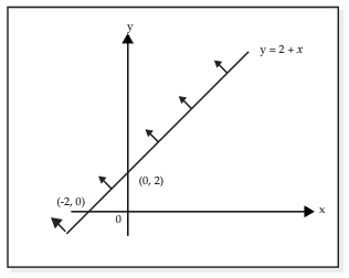 By superimposing the above two graphs we determine the common region ACD in which the pairs (x, y) satisfy both inequalities.

Example 1: We now consider the problem of drawing graphs of the following inequalities
 Note: [1] The inequalities 3x + y ≤ 6 and x – y≤ –2 differ from the preceding ones in that these also include equality signs. It means that the points lying on the corresponding lines are also included in the region.
[2] The procedure may be extended to any number of inequalities.
We note that the given inequalities may be grouped as follows :

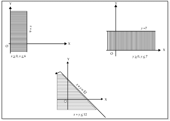
By superimposing the above three graphs, we determine the common region in the xy plane where all the five inequalities are simultaneously satisfied.
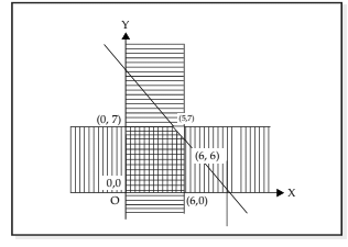
The feasible region, also referred to as the solution set or polygonal convex set, represents a common area defined by constraints in optimization problems. A region is classified as bounded if it can be completely enclosed within a sufficiently large circle. In this context, the shaded area outlined by solid lines in the previous diagram is considered bounded, as it fits within a circle.
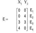
The objective function reaches its maximum or minimum value at one of the corner points, known as extreme points, of the feasible solution. Identifying these extreme points—which are the intersections of the lines that form the boundaries of the region—allows for a compact matrix representation of these points, denoted as E. Additionally, the coefficients of the objective function can be organized into a column vector represented by C. The resulting product matrix EC reveals various values that the objective function can achieve at the different extreme points. The maximum and minimum values of the objective function correspond to the largest and smallest elements in the matrix EC, respectively. The row in this matrix where these values occur indicates the optimal solution, showcasing the pairs of values that yield the best outcome.
In the context of the problem under consideration.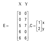
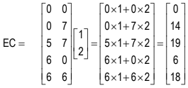
The given objective function viz. Z = x + 2y is maximum at the points (5, 7) present in the third row of the matrix E. Thus the optimal solution is x = 5, y = 7, and the maximum value of the objective function is 19.
We now list the steps to be followed under graphical solution to a linear programming problem.
- Step 1: Identify the area that meets the given inequalities.
- Step 2: Check if the area is bounded. If it is not bounded, it may mean there are hidden conditions that can help define the area, or there may be no solution to the issue.
- Step 3: Create the matrix E that includes the extreme points, and the column vector C for the objective function.
- Step 4: Calculate the product EC. For maximization, find the row in EC with the highest value; for minimization, find the row with the lowest value.
- Step 5: Optimize the objective function based on the elements from the same row in the extreme points matrix E.
Note: If the slope of the objective function matches the slope of one side of the feasible area, there are many possible solutions. However, the best value of the objective function will still be the same.
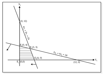
Example 2: A manufacturer produces two products A and B, and has his machines in operation for 24 hours a day. Production of A requires 2 hours of processing in machine M1 and 6 hours in machine M2. Production of B requires 6 hours of processing in machine M1 and 2 hours in machine M2. The manufacturer earns a profit of ₹5 on each unit of A and ₹ 2 on each unit of B. How many units of each product should be produced in a day in order to achieve maximum profit?
Solution:
Let x1 be the number of units of type A product to be produced, and x2 is that of type B product to be produced. The formulation of the L.P.P. in this case is as below:
Maximize Z = 5x1 + 2x2
* It is inconceivable for a practical problem to have an unbounded solution. subject to the constraints.
2x 1 + 6x2< 24
6x1 + 2x2< 24
x1 ≥ 0, x2 ≥ 0
For the line
For the line
The shaded portion in the diagram is the feasible region and the matrix of the extreme points E1, E2, E3 and E4 is
The column vector for the objective function is
The column vector the values of the objective function is given by
Since 21 is the largest element in matrix EC, therefore the maximum value is reached at the extreme point E3 whose coordinates are (3,3).
Thus, to achieve maximum profit the manufacturer should produce 3 units each of both the products A and B.
[Intext Question]
Summary of Graphical Method
- Formulating the linear programming problem: This involves writing the objective function and the constraints in a standardized form.
- Plotting capacity constraints: To do this on graph paper, you typically need two endpoints. This is achieved by assuming that one of the constraints is zero at the same time. If a constraint only involves one factor, the line will have a single starting point and will run parallel to the other axis.
- Identifying the feasible region: This step includes finding the corner points. It is usually done by analyzing the graph, but you can also determine a point by solving the simultaneous equations related to the two lines that intersect at that point.
- Testing corner points for maximum profit: To find out which corner point yields the highest profit, you need to substitute the coordinates of that corner point into the objective function.
- Decision-making regarding resource utilization: Sometimes, it is necessary to check if the optimal point leaves any resources unused. To do this, you need to input the coordinates of the optimal point into the constraints to see which constraints are not fully utilized.
Example 3: A company produces two products A and B, each of which requires processing in two machines. The first machine can be used at most for 60 hours, the second machine can be used at most for 40 hours. The product A requires 2 hours on machine one and one hour on machine two. The product B requires one hour on machine one and two hours on machine two. Express above situation using linear inequalities.
Solution: Let the company produce, x number of product A and y number of product B. As each of product A requires 2 hours in machine one and one hour in machine two, x number of product A requires 2x hours in machine one and x hours in machine two. Similarly, y number of product B requires y hours in machine one and 2y hours in machine two. But machine one can be used for 60 hours and machine two for 40 hours. Hence 2x + y cannot exceed 60 and x + 2y cannot exceed 40. In other words,
2x + y ≤ 60 and x + 2y ≤ 40.
Thus, the conditions can be expressed using linear inequalities.
Example 4: A fertilizer company produces two types of fertilizers called grade I and grade II. Each of these types is processed through two critical chemical plant units. Plant A has maximum of 120 hours available in a week and plant B has maximum of 180 hours available in a week. Manufacturing one bag of grade I fertilizer requires 6 hours in plant A and 4 hours in plant B. Manufacturing one bag of grade II fertilizer requires 3 hours in plant A and 10 hours in plant B. Express this using linear inequalities.
Solution: Let us denote by x1, the number of bags of fertilizers of grade I and by x2, the number of bags of fertilizers of grade II produced in a week. We are given that grade I fertilizer requires 6 hours in plant A and grade II fertilizer requires 3 hours in plant A and plant A has maximum of 120 hours available in a week. Thus 6x1 + 3x2 ≤ 120.
Similarly grade I fertilizer requires 4 hours in plant B and grade II fertilizer requires 10 hours in Plant B and Plant B has maximum of 180 hours available in a week. Hence, we get the inequality 4x1 + 10x2 ≤180.
Example 5: Draw the graph of the solution set of the following inequality and equality:

Mark the common region.
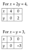
Solution: We draw the graph of both x + 2y = 4 and x – y ≤ 3 in the same plane.
The solution set of system is that portion of the graph of x + 2y = 4 that lies within the half-plane representing the inequality x – y ≤3.
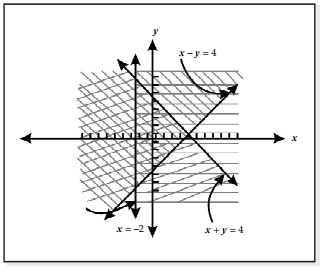
Example 7: Draw the graphs of the following inequalities:
 and mark the common region.
Solution:
The common region is the one represented by overlapping of the shadings.
Example 8: Draw the graphs of the following linear inequalities:
 and mark the common region.
Solution:
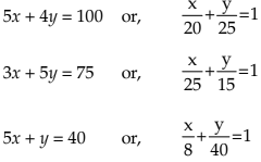
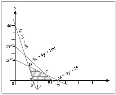
Plotting the straight lines on the graph paper we have the above diagram:
The common region of the given inequalities is shown by the shaded portion ABCD.
Example 9: Draw the graphs of the following linear inequalities:

and mark the common region:
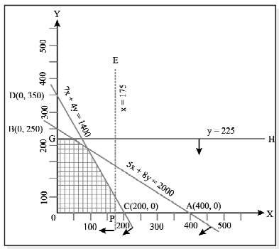
Solution: Let us plot the line AB (5x +8y = 2,000) by joining the points A(400, 0) and B(0, 250).
Similarly, we plot the line CD (7x + 4y = 1400) by joining the points C(200, 0) and D(0, 350).
Also, we draw the lines EF(x = 175) and GH (y = 225).
The required graph is shown alongside in which the common region is shaded.
Example 10: Draw the graphs of the following linear inequalities:

and mark the common region.
Solution:
We plot the line AB (x + y = 1), CD (y = 5), EF (x = 6), DE (7x + 9y = 63).
Given inequalities are shown by arrows.
Common region ABCDEF is the shaded region.
Example 11: Two machines (I and II) produce two grades of plywood, grade A and grade B. In one hour of operation machine I produces two units of grade A and one unit of grade B, while machine II, in one hour of operation produces three units of grade A and four units of grade B. The machines are required to meet a production schedule of at least fourteen units of grade A and twelve units of grade B. Express this using linear inequalities and draw the graph.
Solution: Let the number of hours required on machine I be x and that on machine II be y. Since in one hour, machine I can produce 2 units of grade A and one unit of grade B, in x hours it will produce 2x and x units of grade A and B respectively. Similarly, machine II, in one hour, can produce 3 units of grade A and 4 units of grade B. Hence, in y hours, it will produce 3y and 4y units Grade A & B respectively.
The given data can be expressed in the form of linear inequalities as follows:
2x + 3y ≥ 14 (Requirement of grade A)
x + 4y ≥ 12 (Requirement of grade B)
Moreover x and y cannot be negative, thus x ≥ 0 and y ≥ 0
Let us now draw the graphs of above inequalities. Since both x and y are positive, it is enough to draw the graph only on the positive side.
The inequalities are drawn in the following graph:
For 2x + 3y = 14,
For x + 4y = 12,
In the above graph we find that the shaded portion is moving towards infinity on the positive side. Thus the result of these inequalities is unbounded.
|
101 videos|277 docs|89 tests
|


