Market Equilibrium Chapter Notes | Economics Class 11 - Commerce PDF Download
| Table of contents |
|
| Introduction |
|
| Equilibrium, Excess Demand, and Excess Supply |
|
| Shifts in Demand and Supply |
|
| Market Equilibrium: Free Entry and Exit |
|
| Applications |
|

Introduction
In this chapter, we will build upon the concepts of consumer and firm behaviour as price takers. Recall the following concepts:
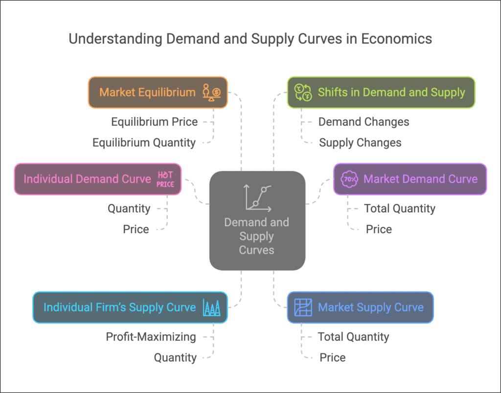
- Individual Demand Curve: This curve shows the quantity of a commodity a consumer is willing to buy at different prices when they take the price as given.
- Market Demand Curve: Represents the total quantity of a commodity all consumers are willing to purchase at different prices when they all take the price as given.
- Individual Firm’s Supply Curve: Indicates the quantity of a commodity a profit-maximizing firm would like to sell at different prices when it takes the price as given.
- Market Supply Curve: This curve shows the total quantity of a commodity all firms are willing to supply at different prices when each firm takes the price as given.
- Market Equilibrium: The point where the market demand and supply curves intersect, determining the equilibrium price and quantity.
- Shifts in Demand and Supply: Examining how changes in demand and supply affect the equilibrium price and quantity.
Equilibrium, Excess Demand, and Excess Supply
- A perfectly competitive market is made up of buyers and sellers who act in their own self-interest. Consumers aim to maximize their preferences, while firms strive to maximise their profits. These objectives align in equilibrium.
- Equilibrium is a state where the plans of all consumers and firms in the market match, leading to a market clearance. In this state, the total quantity that firms want to sell equals the quantity that consumers want to buy, meaning market supply equals market demand.
- The price at which equilibrium occurs is known as the equilibrium price, and the quantity bought and sold at this price is called the equilibrium quantity.
- Mathematically, (p*, q*) represents equilibrium if qD(p*) = q S(p*), where p* is the equilibrium price, qD(p*) is market demand, and qS(p*) is market supply at price p*.
- When market supply exceeds market demand at a certain price, it results in excess supply. Conversely, when market demand surpasses market supply at a price, it leads to excess demand.
- Therefore, equilibrium in a perfectly competitive market can also be described as a situation of zero excess demand and zero excess supply.
- Whenever market supply does not equal market demand, indicating a lack of equilibrium, there will be a tendency for the price to change.
Out-of-Equilibrium Behaviour
- Since the time of Adam Smith, it has been thought that in a market with perfect competition, there exists an ‘Invisible Hand’ that helps to adjust prices when there are imbalances in the market.
- This ‘Invisible Hand’ is believed to increase prices when there is excess demand and to decrease prices when there is excess supply.
- Throughout our analysis, we will keep in mind that this ‘Invisible Hand’ is very important for achieving market equilibrium.
- We will assume that the ‘Invisible Hand’ can reach this balance through its actions, and we will stick to this idea during our discussion.
Market Equilibrium with a Fixed Number of Firms
In a perfectly competitive market with a fixed number of firms, the market equilibrium is determined by the intersection of the market supply and demand curves. The market supply curve (SS) represents the quantity of a commodity that firms are willing to supply at different prices, while the market demand curve (DD) shows the quantity that consumers are willing to purchase at various prices.
Equilibrium occurs at the point where these two curves intersect, indicating that the quantity supplied equals the quantity demanded. This point is characterized by the equilibrium price (p*) and equilibrium quantity (q*). At prices above p*, there is excess supply, while at prices below p*, there is excess demand.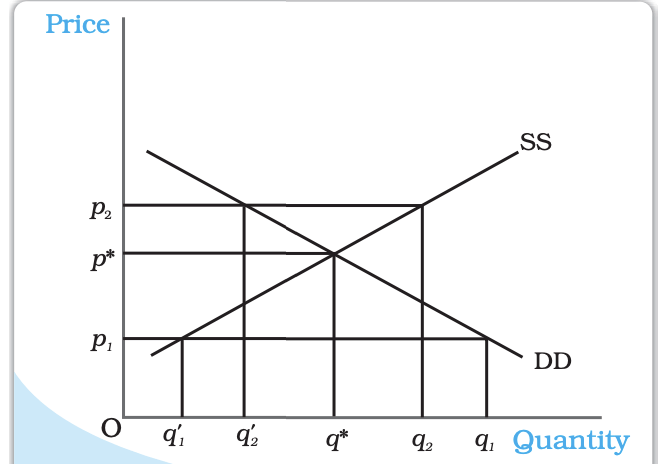
When the market is not in equilibrium, adjustments occur. For instance, if the price is set at p1, resulting in excess demand (where quantity demanded exceeds quantity supplied), the price tends to rise as consumers are willing to pay more. Conversely, if the price is at p2, leading to excess supply (where quantity supplied exceeds quantity demanded), firms will lower their prices. These adjustments continue until the market reaches equilibrium at price p* and quantity q*.
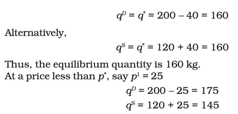
To illustrate this concept, consider an example of a market for wheat with a specific demand and supply curve. The equilibrium price and quantity can be calculated by setting the demand equal to the supply and solving for the price.
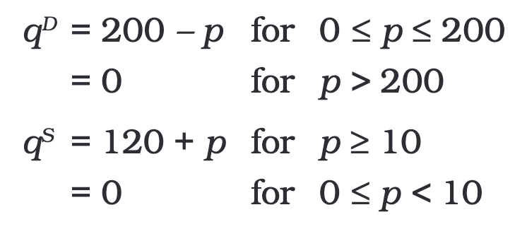
where qD and qS denote the demand for and supply of wheat (in kg) respectively and p denotes the price of wheat per kg in rupees. Since at equilibrium, the price market clears, we find the equilibrium price(denoted by p*) by equating market demand and supply and solving for p*.
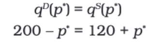
Rearranging and solving for p:
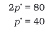
The equilibrium price of wheat is Rs 40 per kg. The equilibrium quantity (represented as q*), is found by substituting the equilibrium price into either the demand or supply curve equation. At equilibrium, the quantity of wheat that is demanded is equal to the quantity that is supplied.
Wage Determination in the Labour Market
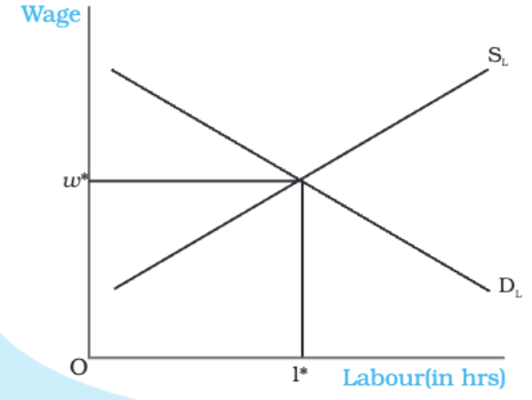
In a perfectly competitive market, the wage is determined by the intersection of the demand and supply curves for labour.
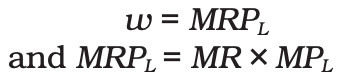
The demand for labour by a firm is based on the Marginal Revenue Product of Labour (MRPL), which is the additional revenue generated by employing one more unit of labour.
Firms will continue to hire labour until the MRPL equals the wage rate (w).
In a perfectly competitive market, the MRPL is equal to the Value of Marginal Product of Labour (VMPL), since marginal revenue is the same as the price of the output. This can be represented as:
The supply of labour is determined by households, who make a trade-off between leisure and income.
As the wage rate increases, individuals are willing to supply more labour, leading to an upward-sloping supply curve.
The market demand curve for labour is derived by aggregating the individual firms’ demand curves, which are downward sloping.
- We now focus on the supply side.
- As mentioned before, households decide how much labor to provide based on the wage rate.
- Their decision is really about choosing between income and leisure.
- On one side, people enjoy leisure and often find work to be a hassle.
- On the other side, they value the income that comes from working.
- This creates a trade-off between enjoying leisure time and working more hours.
- To understand the labor supply curve for one person, let’s assume at a wage of w1, the individual provides l1 units of labor.
- If the wage increases to w2, there will be two main effects:
- First, with the wage increase, the opportunity cost of leisure also goes up, making leisure more expensive. Therefore, the individual may want to enjoy less leisure time.
- Second, as the wage rises to w2, the individual’s purchasing power increases, making them more likely to spend on leisure activities. - The final impact of the wage increase depends on which of these two effects is stronger.
- At low wage rates, the first effect (wanting to work more) is stronger, so the individual will supply more labor when wages rise.
- However, at high wage rates, the second effect (wanting to enjoy more leisure) takes over, leading the individual to supply less labor as wages increase.
- This results in a backward-bending labor supply curve, which shows that up to a certain wage, the supply of labor increases with wage rises.
- Beyond this point, as wages continue to rise, the supply of labor decreases.
- Yet, when looking at the overall market, the market supply curve for labor, created by adding up individual supplies at various wages, will still slope upward.
- This is because even if some individuals decide to work less at higher wages, many others will be drawn to offer more labor.
- With an upward-sloping supply curve and a downward-sloping demand curve, the equilibrium wage rate is found at the point where these two curves meet.
- This intersection represents the balance between the labor that households want to supply and the labor that firms want to hire.
Work-Leisure Trade-Off
Effect of Increased Cost of Leisure: When the cost of leisure increases, individuals tend to enjoy less leisure time because it becomes more expensive. As a result, they are inclined to work longer hours.
Impact of Wage Increase (from w1 to w2): An increase in the wage rate to w2 enhances the purchasing power of individuals, leading them to desire more leisure activities.
Predominance of Effects: The overall impact of a wage increase depends on which effect is stronger:
- At low wage rates, the desire for more leisure (due to increased purchasing power) is weaker, so individuals are willing to supply more labour when wages increase.
- At high wage rates, the desire for more leisure becomes stronger, and individuals may choose to supply less labour as wages rise.
Backward-Bending Labour Supply Curve:
- Explanation: This curve illustrates that up to a certain wage rate, an increase in wages leads to an increased supply of labour. Beyond this wage rate, further increases in wages may result in a decreased supply of labour.
- Example: For instance, at lower wage rates, individuals are more willing to work longer hours as wages increase. However, at higher wage rates, individuals may prefer to enjoy more leisure time, even if wages continue to rise.
Market Supply Curve of Labour:
- Aggregation of Individual Supply: The market supply curve is obtained by aggregating the supply of labour from individuals at different wage levels.
- Upward-Sloping Nature: Despite some individuals choosing to work less at higher wages, the overall supply of labour increases because more individuals are attracted to supply labour at higher wage levels.
Determination of Equilibrium Wage Rate:
- Intersection of Supply and Demand Curves: The equilibrium wage rate is determined at the point where the upward-sloping supply curve intersects the downward-sloping demand curve.
- Equality of Labour Supply and Demand: This point represents the situation where the quantity of labour that households are willing to supply equals the quantity of labour that firms wish to hire.
Shifts in Demand and Supply
- In the previous section, we looked at market equilibrium while assuming that certain factors remain unchanged. These factors include consumer tastes and preferences, prices of related goods, consumer incomes, technology, market size and input prices used in production.
- However, if any of these factors change, it can cause either the supply curve or the demand curve, or both, to shift. This shift will influence the equilibrium price and quantity in the market.
- First, we will develop a general theory that explains how these shifts affect equilibrium.
- Then, we will examine how changes in some of the factors mentioned above can impact equilibrium.
Demand Shift
- Consider the image below that shows how a change in demand affects the market when the number of companies stays the same.
- The starting point of balance in the market is called E, where the demand curve DD0 meets the supply curve SS0.
- At this point E, the quantity of goods sold is q0 and the price of those goods is p0.
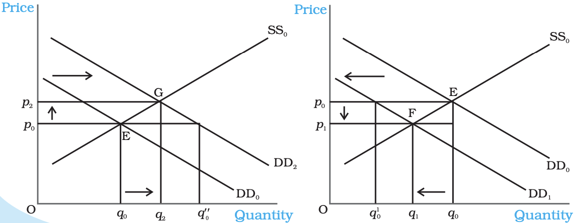
- When the market demand curve moves to the right (to DD2) while the supply curve stays the same (SS0), it means that at any price, people want to buy more than before.
- At the price level of p0, there is now a situation of excess demand equal to q0 q''0.
- Because of this excess demand, some people will be willing to pay a higher price, which will cause the price to go up.
- A new equilibrium is reached at point G, where the new equilibrium quantity q2 is greater than the old quantity q0, and the new equilibrium price p2 is higher than p0.
- On the other hand, if the demand curve shifts to the left (to DD1), it indicates that at any price, the quantity demanded is now less than before.
- Therefore, at the original equilibrium price p0, there will be excess supply equal to q'0q0.
- In response to this excess supply, some businesses will lower their prices to sell their goods.
- The new equilibrium occurs at point F, where the demand curve DD1 intersects the supply curve SS0, resulting in a new equilibrium price p1 that is lower than p0 and a quantity q1 that is less than q0.
- It’s important to note that the direction of change in both equilibrium price and quantity is the same whenever the demand curve shifts.
- After discussing the general theory, we can look at specific examples to see how the demand curve and the equilibrium quantity and price are affected by various factors mentioned in Chapter 2.
- For instance, if consumers receive a salary increase, their incomes will rise. This leads to a change in equilibrium.
- With higher incomes, consumers can spend more on certain goods. However, remember that for inferior goods, demand decreases as income increases, while for normal goods, demand increases as income rises.
- Taking clothes as an example of a normal good, an increase in consumer income results in higher demand, shifting the demand curve from DD0 to DD2.
- The supply curve remains unchanged, as it is only affected by factors related to production costs or technology.
- As illustrated in the figure, the new equilibrium reflects a higher price for clothes and an increase in the quantity demanded and sold.
- Now consider another example where the number of consumers in the clothes market increases.
- With more consumers, assuming all other factors remain the same, at each price, the demand for clothes rises.
- This increase in the number of consumers will again shift the demand curve to the right, similar to the previous case.
- However, this change does not affect the supply curve, which only shifts due to changes in the behavior of firms or an increase in the number of firms, as explained in Chapter 4.
- Again, Figure 5.2(a) shows the rightward shift of the demand curve from DD0 to DD2, while the supply curve at SS0 remains the same.
- This shift results in a new equilibrium point G, where both the price and the quantity demanded and supplied increase compared to the old equilibrium point E.
Supply Shift
Impact of Shift in Supply Curve
- Leftward Shift: When the supply curve shifts leftward (from SS0 to SS2) while the demand curve remains constant, it indicates a decrease in supply at all price levels. This leads to a new equilibrium (point G) where the price increases (to p2) and the quantity sold decreases (to q2).
- Rightward Shift: Conversely, a rightward shift in the supply curve (from SS0 to SS1), with the demand curve unchanged, signifies an increase in supply. This results in a new equilibrium (point F) where the price decreases (to p1) and the quantity sold increases (to q1).
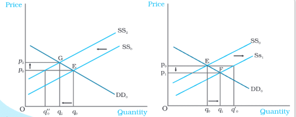
Factors Affecting Supply Shift
- Increase in Input Prices: When the price of an input used in production increases, the marginal cost of production rises. This leads to a leftward shift in the supply curve (from SS0 to SS2), as producers are willing to supply less at each price level. The demand curve remains unchanged (at DD0) because consumer demand is not directly affected by input prices. The result is a higher market price and a lower quantity produced compared to the initial equilibrium.
- Increase in Number of Firms: An increase in the number of firms in the market leads to an increase in supply at each price level, causing a rightward shift in the supply curve (from SS0 to SS1). The demand curve remains unchanged (at DD0). This shift results in a lower market price and an increased quantity produced compared to the initial situation.
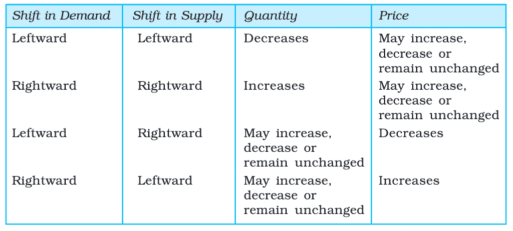
Simultaneous Shifts of Demand and Supply
- Both Demand and Supply Shift Rightwards: Equilibrium quantity increases, but the effect on equilibrium price can vary (increase, decrease, or unchanged) depending on the magnitude of the shifts.
- Both Demand and Supply Shift Leftwards: Equilibrium quantity decreases, and the effect on equilibrium price can vary.
- Demand Shifts Rightward and Supply Shifts Leftward: Equilibrium quantity is ambiguous, but equilibrium price increases.
- Demand Shifts Leftward and Supply Shifts Rightward: Equilibrium quantity is ambiguous, but equilibrium price decreases.
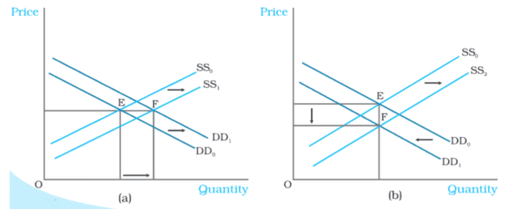
- Initially, the balance is at E, where the demand curve DD0 and the supply curve SS0 meet.
- In panel (a):
- Both the supply and demand curves move to the right.
- The price stays the same, but the equilibrium quantity increases.
- In panel (b):
- The supply curve shifts to the right.
- The demand curve moves to the left.
- The quantity remains unchanged, but the equilibrium price decreases.
Market Equilibrium: Free Entry and Exit
In the previous section, we examined market equilibrium with a fixed number of firms. Now, we will explore market equilibrium when firms can enter and exit the market freely, assuming all firms are identical for simplicity.
Implications of Free Entry and Exit
- The assumption of free entry and exit implies that, in equilibrium, no firm earns supernormal profit or incurs a loss by remaining in production.
- This means that the equilibrium price will be equal to the minimum average cost (AC) of the firms.

To understand this concept better, let's consider two scenarios:
Scenario 1: Supernormal Profit
- If firms are earning supernormal profits at the prevailing market price, new firms will be attracted to enter the market.
- As new firms enter, the supply curve shifts to the right while demand remains unchanged, causing the market price to fall.
- This process continues until supernormal profits are eliminated.
Scenario 2: Less than Normal Profit
- If firms are earning less than normal profit at the prevailing price, some firms will exit the market.
- This exit will lead to an increase in price, and with a sufficient number of firms remaining, the profits of each firm will rise to the level of normal profit.
Equilibrium Price and Quantity
- In equilibrium, the price will be equal to the minimum average cost, ensuring that each firm earns a normal profit.
- The quantity supplied will be determined by market demand at this price, ensuring that the quantity demanded and quantity supplied are equal.
Price Determination with Free Entry and Exit
- In a perfectly competitive market with free entry and exit, the equilibrium price is always equal to the minimum average cost (min AC).
- The equilibrium quantity is determined at the intersection of the market demand curve (DD) with the price line (p = min AC).
Example: Wheat Market
- Demand Curve:. D = 200 - p (for 0 ≤ p ≤ 200), q D = 0 (for p > 200)
- Supply Curve of a Single Firm:. s = p - 10 (for p ≥ 20), q s = 0 (for 0 ≤ p < 20)
Equilibrium Price and Quantity:
- The minimum average cost is Rs. 20, which is the price at which firms will operate.
- At this price, the market demand is 180 kg, and each firm supplies 30 kg.
- The equilibrium number of firms is 6.
Shifts in Demand
- We will explore how changes in demand affect the equilibrium price and quantity when firms can easily enter and exit the market.
- As discussed earlier, when firms can enter and exit freely, the equilibrium price will always match the minimum average cost of the firms.
- This means that even if the market demand curve shifts, the market will still provide the required quantity at the same price at the new equilibrium.
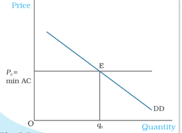
- In the diagram, DD0 represents the initial market demand curve, showing how much consumers want at various prices, while p0 is the price equal to the minimum average cost of the firms.
- The starting equilibrium point is at E, where the demand curve DD0 intersects the p0 = minAC line, with the total quantity demanded and supplied being q0.
- The number of firms in this situation is n0.
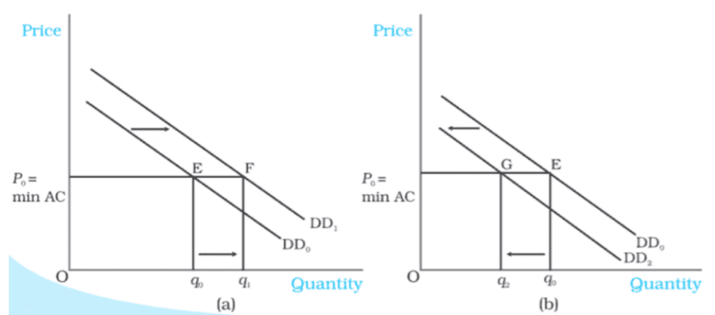
- Now, if the demand curve shifts to the right, there will be excess demand at price p0.
- Some consumers who cannot find the product will be willing to pay a higher price, causing the price to rise.
- This leads to the potential for firms to earn supernormal profits, which will attract new firms into the market.
- The entry of new firms will eliminate these supernormal profits, bringing the price back down to p0.
- At this new equilibrium, a higher quantity, q1, will be supplied at the same price.
- As shown in panel (a), the new demand curve DD1 intersects the p0 = minAC line at point F, resulting in a new equilibrium of (p0, q1) where q1 is greater than q0.
- The new number of firms, n1, will be greater than n0 due to the entry of additional firms.
- Conversely, if the demand curve shifts to the left to DD2, there will be excess supply at price p0.
- Some firms will not be able to sell as much as they want at this price, prompting them to lower their prices.
- This price drop will lead to the exit of some existing firms until the price returns to p0.
- At the new equilibrium, the quantity supplied will decrease to match the reduced demand at that price.
- In panel (b), the shift of the demand curve from DD0 to DD2 shows that quantity demanded and supplied will fall to q2, while the price remains at p0.
- Here, the equilibrium number of firms, n2, is less than n0 due to the exit of some firms.
- Thus, when demand shifts right, the equilibrium quantity and number of firms will increase, whereas a leftward shift will lead to a decrease in both, with the equilibrium price staying the same.
Applications
Government Intervention in Price Control
In this section, we will explore how supply and demand analysis can be applied in real-world situations, particularly focusing on government intervention through price control. Sometimes, the government needs to regulate the prices of certain goods and services when they are either too high or too low compared to the desired levels. We will examine these issues within the framework of perfect competition to understand the impact of such regulations on the market for these goods.
Price Control in Perfect Competition
Perfect competition is a market structure where there are many buyers and sellers, and no single entity has the power to influence prices. In this scenario, we will analyze how government-imposed price controls affect the market dynamics of specific goods and services.
Price Ceiling
A price ceiling is when the government sets a maximum price for certain goods to make them affordable for everyone. This is often applied to essential items like wheat, rice, kerosene, and sugar. Price ceilings are set below the market price because, at the market price, some people wouldn't be able to buy these necessary goods.
For example, let's look at the market for wheat:
- Market Supply and Demand: The supply curve (SS) and demand curve (DD) for wheat determine the equilibrium price (p*) and quantity (q*).
- Imposing a Price Ceiling: When the government sets a price ceiling (cp) below the equilibrium price, it creates excess demand. Consumers want to buy more wheat (qc) than what farmers are willing to supply (cq').
- Resulting Shortage: Even though the government aims to help consumers, the price ceiling can lead to a shortage of wheat.
- Rationing System: To manage this shortage, the government may implement a rationing system. Ration coupons are given to consumers, limiting the amount of wheat each person can buy. This wheat is sold through ration shops or fair price shops.
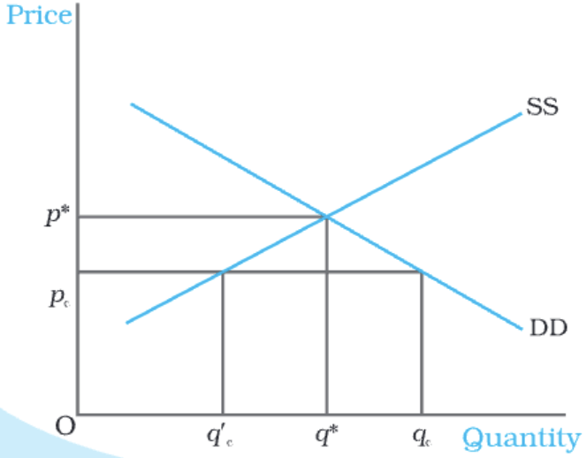
Adverse Consequences of Price Ceiling with Rationing:
- Long Queues: Consumers have to wait in long lines to purchase goods from ration shops.
- Black Market: Some consumers, unsatisfied with the limited quantities from fair price shops, may be willing to pay higher prices, leading to the creation of a black market.
Price Floor
A price floor is a minimum price set by the government for certain goods and services to prevent their prices from falling too low. This is often seen in agricultural price support programs and minimum wage legislation.
- In agricultural price support, the government sets a price floor above the market price to ensure farmers receive a minimum income for their products.
- Similarly, minimum wage laws ensure that workers are paid at least a certain wage, set above the equilibrium wage rate.
- When a price floor is imposed, it creates a situation where the quantity supplied exceeds the quantity demanded, leading to excess supply. For example, if the government sets a price floor (pf) above the equilibrium price (p*), the quantity demanded (qf) will be less than the quantity supplied (q¢ f), resulting in a surplus.
- To manage this surplus, such as in agricultural support, the government may need to purchase the excess supply at the predetermined price.
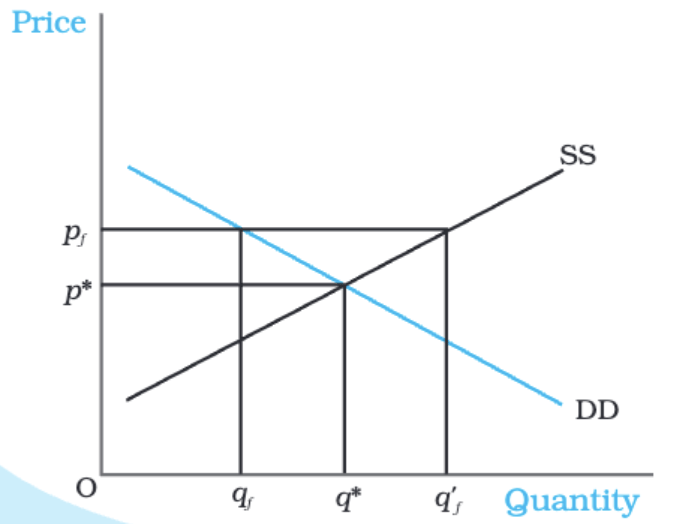
- The figure shows the market supply and demand curves for a commodity where a price floor is set.
- The market would normally balance at a price of p* and a quantity of q*.
- However, when the government establishes a price floor above this equilibrium price, noted as pf, the market demand decreases to qf.
- At the same time, producers wish to supply q′f.
- This situation creates a surplus in the market, calculated as the difference between qf and q′f.
- In agricultural markets, to stop prices from dropping due to this excess supply, the government must purchase the surplus at the set price.
|
59 videos|222 docs|43 tests
|
FAQs on Market Equilibrium Chapter Notes - Economics Class 11 - Commerce
| 1. What is market equilibrium, and why is it important in economics? |  |
| 2. What are excess demand and excess supply? | |
| 3. How do shifts in demand and supply affect market equilibrium? | |
| 4. What role does free entry and exit play in market equilibrium? | |
| 5. Can you provide an example of how market equilibrium can change due to external factors? | |


study material
,video lectures
,Market Equilibrium Chapter Notes | Economics Class 11 - Commerce
,mock tests for examination
,shortcuts and tricks
,Objective type Questions
,Exam
,Important questions
,Extra Questions
,Market Equilibrium Chapter Notes | Economics Class 11 - Commerce
,Free
,Viva Questions
,practice quizzes
,Semester Notes
,Previous Year Questions with Solutions
,past year papers
,Market Equilibrium Chapter Notes | Economics Class 11 - Commerce
,MCQs
,ppt
,Summary
,Sample Paper
;


Chapter Notes: Market Equilibrium Free PDF Download
Importance of Chapter Notes: Market Equilibrium
Chapter Notes: Market Equilibrium
Chapter Notes: Market Equilibrium Commerce Questions
Study Chapter Notes: Market Equilibrium on the App
|
© EduRev
|
Education Revolution
|


|


