Overview: Contextual Applications of Differentiation Chapter Notes | Calculus AB - Grade 9 PDF Download
| Table of contents |
|
| Prerequisites for Success |
|
| What Does a Derivative Represent? |
|
| One-Dimensional Motion |
|
| Related Rates |
|
| Approximating Functions |
|
| L’Hôpital’s Rule |
|
| Wrapping Up |
|

Now that you’ve got the hang of differentiation rules and formulas, it’s time to put them to work! This guide explores how to apply derivative techniques in various scenarios, from motion to related rates and function approximations. Let’s dive into the practical side of calculus!
Prerequisites for Success
To tackle this section, you’ll need a solid grasp of the following concepts:
- Average vs. Instantaneous Rate of Change: Understand the difference between the average rate of change (over an interval) and the instantaneous rate of change (at a specific point).
- Differentiation Techniques:
- Power Rule
- Product Rule
- Quotient Rule
- Chain Rule
- Implicit Differentiation
- Functions to Differentiate:
- Trigonometric Functions
- Inverse Trigonometric Functions
- Inverse Functions
- Logarithmic Functions
- Exponential Functions
- Geometric Formulas:Be familiar with formulas from earlier math courses, including:
- Area
- Volume
- Perimeter
- Circumference
- Pythagorean Theorem
What Does a Derivative Represent?
A derivative captures the instantaneous rate of change of a function, which is also the slope of the tangent line at a given point. While we’ve mostly worked in the xy-plane, derivatives can be applied in diverse contexts. By the end of this section, you’ll be equipped to use derivatives to solve problems beyond the xy-plane!
One-Dimensional Motion
In AP Calculus, we focus on motion along a single axis (one-dimensional motion), with time as the second dimension. Imagine a particle moving left or right along the x-axis, possibly speeding up, slowing down, or reversing direction. We might want to determine its velocity, speed, or whether it’s accelerating.
How might we model this problem? Suppose the position of the particle is given by some function of time x(t). If you just wanted to find the average velocity of the particle over some time interval t1 to t2, we just calculate the change in position (given by the position function) and divide it by the change in time, to get
 From this intuition, you might be able to guess that the instantaneous velocity (over an infinitesimal change in time) will be dx/dt.
The instantaneous velocity will always be signed. We usually define right as the positive direction and left as the negative direction, so if we get that dx/dt = -3 for some value of t, we know that the particle is moving at speed 3 to the left. If we want just the speed, then we use the magnitude of the velocity, which for one-dimensional motion is ∣v∣ = 3.
If we just know the velocity at some instant, we can’t really tell if the particle is speeding up or slowing down. To answer that question, we need to know the acceleration. The acceleration is the rate of change of velocity dv/dt meaning that if velocity is increasing over time, there is positive acceleration, and if velocity is decreasing over time, there is negative acceleration. What if the acceleration is 0? That means that the particle is moving at a constant rate.
To summarize:
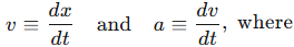
where x(t) is the position function of the object, v is the velocity, and, a is the acceleration.
Related Rates
We use related rates when the rate of one thing happening is dependent on the rate of another thing happening. A very common example is considering how fast the volume or area of an object changes if the radius, height, etc. is changing at a certain rate. The best way to learn how to do related rates problems is to just do a lot of them! Every problem will be a little different, and the challenge is in modeling the problem — not necessarily doing the calculations.
Here is an easy example to get a feel for what you will have to do. Suppose you are blowing a bubble, which is perfectly spherical, and the radius of the bubble increases at a constant rate of 15 mm/s. How fast is the volume increasing?
Since we want to find how fast the volume is increasing, we want to find dV/dt. Now,
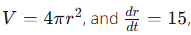 so we have:
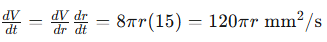
Now, we might be asked how much the volume of the bubble is increasing after blowing it for 2 seconds. We will assume that when t = 0, the bubble has radius 0, so when t = 2, the bubble will have radius 30 mm. So, the volume is increasing at 3600π mm2/s = 36π cm2/s.
There are many other examples of related rates problems. Don’t be scared if the function has more than one variable! Try not to overcomplicate things — keep the variable that you need and rewrite the missing variable in terms of the variables you have. For example, if you want to find dV/dt for a cone and you are given dr/dt, but not dh/dt then you can find h in terms of r and V.
Approximating Functions
Sometimes, you need to approximate a complex function with a simpler linear one, especially in fields like statistics or machine learning. If a linear function y is tangent to a function f at a point (x₀, y₀), you can use it to approximate f(x) for x values close to x₀.
For AP Calculus, you’ll typically approximate values within 0.1 or 0.2 units of x₀. To determine if the approximation underestimates or overestimates:
- If the function is concave up at x₀, the tangent line lies below the function, leading to an underestimate.
- If concave down, the tangent line is above, leading to an overestimate.
L’Hôpital’s Rule
When evaluating limits that result in indeterminate forms like 0/0 or ±∞/∞, L’Hôpital’s Rule is a handy tool. It states:
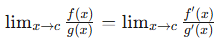
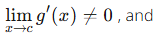
if the following necessary conditions are met:
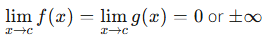
- f(x) and g(x) are differentiable on an open interval I except for possibly at point c ∈ I. This means that both functions are differentiable everywhere around c, but they may or may not be differentiable around c.
Some of these conditions seem obvious, while others may not be. In order to get some intuition about why we might need for these conditions to be met, we will show L’Hospital’s rule in the case where 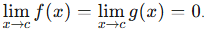 If we assume all of the other necessary conditions, then
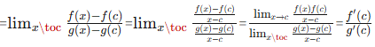 Now, we can see that if
 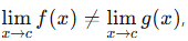 L’Hopital’s probably won’t work, and if f(x) and g(x) are not differentiable around c, then this method also won’t work.
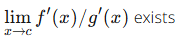
A useful corollary to L’Hopital’s rule is that if f is a function that is continuous at aa and f′(x) exists for all values in an open interval containing a (except for maybe x = a), then if  exists, then.
Wrapping Up
By mastering these applications—motion, related rates, function approximation, and L’Hôpital’s Rule—you’ll be ready to tackle a wide range of calculus problems. Practice these concepts, and you’ll see how derivatives bring math to life in real-world scenarios!
|
26 videos|75 docs|38 tests
|
FAQs on Overview: Contextual Applications of Differentiation Chapter Notes - Calculus AB - Grade 9
| 1. What is the concept of a derivative in calculus? |  |
| 2. How do derivatives apply to one-dimensional motion? | |
| 3. What are related rates in calculus? | |
| 4. How can I approximate functions using derivatives? | |
| 5. What is L'Hôpital's Rule and when do you use it? | |


video lectures
,mock tests for examination
,Extra Questions
,past year papers
,practice quizzes
,Overview: Contextual Applications of Differentiation Chapter Notes | Calculus AB - Grade 9
,Overview: Contextual Applications of Differentiation Chapter Notes | Calculus AB - Grade 9
,Exam
,Summary
,shortcuts and tricks
,study material
,Important questions
,Overview: Contextual Applications of Differentiation Chapter Notes | Calculus AB - Grade 9
,Sample Paper
,Free
,Previous Year Questions with Solutions
,Objective type Questions
,Semester Notes
,ppt
,Viva Questions
,MCQs
;


Chapter Notes: Overview: Contextual Applications of Differentiation Free PDF Download
Importance of Chapter Notes: Overview: Contextual Applications of Differentiation
Chapter Notes: Overview: Contextual Applications of Differentiation
Chapter Notes: Overview: Contextual Applications of Differentiation Grade 9 Questions
Study Chapter Notes: Overview: Contextual Applications of Differentiation on the App
|
© EduRev
|
Education Revolution
|


|


