Concepts of Macroeconomics (Part - 1) - Macroeconomics | Macro Economics - B Com PDF Download
Assessment of prior Knowledge
Macroeconomics is formed by combining two words: Macro and Economics. The term "Macro" comes from the Greek word "Uakpo", meaning large, while Economics refers to the study of production, consumption, and distribution of goods and services. Therefore, Macroeconomics focuses on the overall economic system, analyzing total production, total consumption, and total distribution rather than individual transactions.
Development of Macroeconomic Thought
- Adam Smith, the father of modern economics, suggested that if individuals focused solely on their self-interest, there would be no need to analyze national income, wealth, or economic welfare.
- Initially, economists believed that markets did not exist within an economy. Later, they accepted the presence of markets but argued that equilibrium could not be determined simply through supply and demand.
- Eventually, economists recognized the influence of microeconomic variables on the overall economy, highlighting the need to study economic systems at a broader level.
Evolution of Macroeconomic Theories
- Macroeconomics emerged during the 16th and 17th centuries with the ideas of the Mercantilists.
- Economists like Cassel, Marshall, Pigou, and Hayek later contributed to theories on money and price levels.
- During the Great Depression, John Maynard Keynes introduced a new perspective on macroeconomics through his book The General Theory of Employment, Interest, and Money (1936).
- Keynes argued that declining demand for goods and services leads to unemployment and a lower GDP, making it necessary to rethink economic policies.
- His ideas, known as Keynesian Economics, provided a foundation for modern macroeconomic policies.
Impact of Keynesian Economics
- Keynes’ theories highlighted the importance of government intervention in stabilizing the economy.
- The decline in demand for goods and services during an economic downturn leads to higher unemployment and slower economic growth.
- Keynes explained these concepts extensively in his work, shaping how economists approach national economic planning.
- Following Keynes, several economists expanded macroeconomic theories, exploring different approaches to understanding economic fluctuations.
- Macroeconomics continues to evolve, focusing on factors that influence national economies, including growth, stability, and overall welfare.
Definitions of Macroeconomics
- According to R.G.D. Allen, “The term Macroeconomics applies to the study of relations between broad economics aggregates.”
- According to Edward Shapiro, “The major task of macroeconomics is the explanation of what determines the economy’s aggregate output of goods and services. It deals with the functioning of the economy as a whole”.
- According to Ackley Gardner, "Macroeconomics concerns with such variables as the aggregate volume of the output of an economy, with the extent to which its resources are employed, with the size of national income and with the general price level".
Scope of Macroeconomics
I. Theory of National Income
Macroeconomics studies the measurement and methods of calculating national income. This includes aggregate saving, aggregate consumption, and aggregate investment.
II. Theory of International Trade
International trade involves the exchange of goods and services between countries, impacting the entire economy. Thus, it is a key area of macroeconomic study.
III. Theory of Employment
The study of employment levels, different types of unemployment, and the causes behind unemployment falls under the scope of macroeconomics.
IV. Theory of General Price Level
The general price level is influenced by business cycles. Inflation and deflation are two major factors analyzed under macroeconomics.
V. Theory of Money
Macroeconomics examines various theories of money, its role in the economy, and the effects of government income and expenditure on economic stability.
VI. Theory of Trade Cycles
Trade cycles represent fluctuations in the market, including periods of economic growth and decline. Since these cycles impact the overall economy, they are studied in macroeconomics.
VII. Theory of Economic Growth
Macroeconomic theories are applied to ensure balanced economic growth, which is a major objective in economic policy formulation.
Importance of Macroeconomics
1. Aid in Formulating Economic Policies
Macroeconomics focuses on the economy as a whole, analyzing aggregate economic factors. Government policies are designed considering the overall economic conditions. For instance, during an economic downturn, it becomes crucial to study the causes of recession and rising unemployment. Macroeconomic analysis helps in identifying these causes and provides insights for policy formulation, making it an essential tool for economic planning.
2. Understanding the Functioning of an Economy
Macroeconomics examines key economic concerns such as total output, income, employment, and price levels. A thorough understanding of these aggregate variables is essential for ensuring economic stability. Since every nation strives for smooth economic operations, macroeconomic studies help in analyzing and addressing complex economic challenges.
3. Determining National Income
National income is a significant macroeconomic concept, as it serves as an indicator of a nation's overall performance. Assessing national income helps in tackling issues like overproduction and unemployment. The data collected on national income aids in predicting economic activities and understanding income distribution across various sectors.
4. Contribution to Economic Growth
Since macroeconomics assists in forming economic policies, these policies play a crucial role in ensuring stable and long-term economic growth. Theories related to unemployment, price fluctuations, and national income help in addressing these economic challenges, making macroeconomics an essential aspect of economic development.
5. Role in the Development of Microeconomics
Macroeconomic analysis provides a foundation for understanding microeconomics. Without knowledge of aggregate economic data, microeconomic principles cannot be effectively developed. For instance, the behavior of an individual firm does not represent the entire industry. Instead, macroeconomic studies help in analyzing collective market behavior, thereby contributing to the evolution of microeconomic theories.
6. Importance in Economic Planning
Economic planning is necessary for achieving balanced economic development and addressing various economic challenges. Designing effective economic plans requires expertise in macroeconomic concepts such as sectoral interdependence, national income composition, and employment levels. Thus, macroeconomics plays a key role in formulating and executing economic plans.
7. Understanding Trade Cycles
Trade cycles represent fluctuations in economic activity, including phases like boom, recession, and recovery. These fluctuations can be better understood through macroeconomic analysis. Studying key factors such as aggregate demand, consumption, and production helps in addressing trade cycle variations. Macroeconomics enables policymakers to develop strategies for managing inflation and deflation, ensuring business stability.
8. Addressing Monetary Issues
Macroeconomics covers crucial topics such as money, monetary theories, banking systems, and credit policies. Economists rely on macroeconomic insights to analyze these monetary components and propose solutions to financial challenges. Frequent changes in a country’s monetary system can have adverse effects, which can be mitigated using appropriate macroeconomic measures.
9. Analyzing Unemployment
Unemployment is a critical issue, particularly in developing nations. During economic downturns, understanding labor market requirements becomes essential. The Keynesian theory of employment, developed through macroeconomic studies, provides insights into employment levels based on aggregate demand and labor supply. Macroeconomics helps in identifying the causes, consequences, and solutions for unemployment.
By studying macroeconomic principles, policymakers and economists can formulate strategies for sustainable economic development, ensuring economic stability and growth.
Types of Macroeconomic
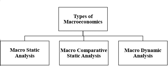
I. Macro static analysis
The term "static" carries different meanings across various fields of study. In economics, it refers to a state where movement occurs at a specific level without any change. According to Clark, a static state is one where five key factors remain unchanged: population size, capital supply, production methods, business organization forms, and consumer wants. Despite these constants, the economy continues to function at a steady pace, ensuring certainty in the system. Professor Kurihara describes macro static as a still image of the economy, capturing its state without any fluctuations.
Macro static represents the static equilibrium position of the economy. Whenever an economy is working at equilibrium point E and it is producing at a constant rate without any change in the other variables, it is known as static state of economy at a point of time. This equilibrium is shown through a timeless identity equation without any adjusting mechanism:

Here,
Y= Total Income
C= Total Consumption
I= Total Investment
According to static Keynesian model, the interaction of aggregate supply function and the aggregate demand function are helpful to determine the level of National Income. This model includes the above identity equation to represent the equilibrium in the economy. This model is shown in figure 2 as under:
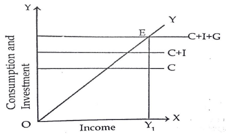
Here, 45º line represents the aggregate supply function,
- C+I+G line represent the aggregate demand function
- E the intersection point represents point of effective demand through which level of National income (OY) is shown.
Thus, macro static refers to timeless economy. It cannot be formed or destroyed. This is an equilibrium situation. This situation cannot be changed whether the previous position and subsequent position of the economy change or not.
II. Macro dynamic analysis
Macro dynamic analysis studies the cause of change in two equilibrium points. It analyses the process of change which continues over a period of time. An economy may change over a period of time in two major ways:
(a) Without changing its pattern
(b) By changing its pattern
Macro dynamic analysis focuses on the second type of change, which occurs due to shifts in factors such as population, capital, production techniques, business organization structures, and consumer preferences. This analysis examines the forces driving these changes within an economy. It takes into account time lags, rates of change, and both past and anticipated values of economic variables. As Kurihara explains, "Macro-dynamics examines discrete movements or rates of change in macroeconomic variables, allowing us to view the economy as a continuously evolving system, much like a motion picture." The following diagram shows the operation of analysis:
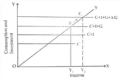
This diagram represents the change of equilibrium from point E to E1 which shows change in government expenditure. This is not a sudden change but it has been increased by a process and time-lag. This process can be understood as the government increase investment which might have result in more employment, high productivity and high level of income. Thus, macro dynamic analysis is a method to describe the causes behind the change in economy due to change in other variables over a period of time.
III. Macro comparative static analysis
Macro comparative static analysis was first introduced by German economist F. Oppenheimer in 1916 as a method of economic analysis. According to Schumpeter, “Whenever we examine the impact of a disturbance on a given state by identifying the static conditions before and after the disturbance has influenced the system, this approach is called Comparative Statics.” In other words, comparative static analysis involves comparing different equilibrium states. In macro static analysis, equilibrium remains fixed at a specific point, denoted as E, at a particular moment in time. In contrast, macro dynamic analysis illustrates a shift in equilibrium from point E to E1. Macro comparative static analysis focuses on studying changes in equilibrium positions from E to E1 as a result of specific variations in other economic variables. Detailed analysis of macro comparative analysis is shown through a figure as under:
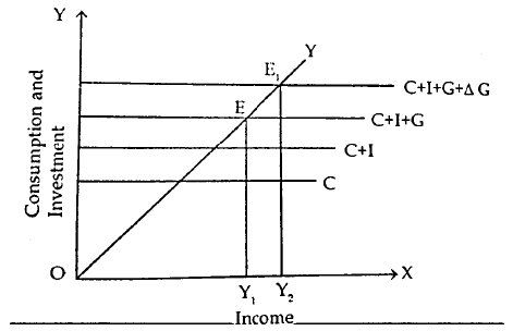
The initial point of equilibrium is at point E where Y (Total income) and C+I+G (total consumption, total investment and government expenditure) intersect each other. But after the inducement of government expenditure the equilibrium point shift from E to E1. New equilibrium point E1 is situated at the intersection of Y and C+I+G+∆G. At this level total income shifts from OY1 to OY2. Thus, the study between two equilibrium points is known as Macro Comparative Static Analysis.
Macro comparative static analysis has some drawbacks also. These are discussed as under:
(a) It ignores the problems related with economic fluctuations.
(b) This method explains only the process of change from one position to another position of equilibrium. Complete reasons behind this change are not cleared under this method.
(c) This method neglects the transitional period.
Variables of Macroeconomics
I. Aggregate Demand
- Demand represents the quantity of goods and services that consumers are willing and able to purchase at different price levels over a specific period. Aggregate demand, however, refers to the total expenditure on all finished goods and services within an economy during an accounting year. It is defined as the total monetary spending on goods and services at a given price level at a specific point in time.
II. Aggregate Supply
- Supply denotes the quantity of goods and services that producers are willing to offer for sale at different price levels over a period, assuming other factors remain unchanged. Aggregate supply refers to the overall production or total supply of goods and services in an economy within an accounting period.
III. Aggregate Consumption
- Aggregate consumption is the total amount spent on goods and services by all consumers in an economy during a given accounting period.
IV. Aggregate Investment
- Investment refers to the acquisition of assets that contribute to an increase in income over time. In economics, it is defined as the expenditure made by producers to acquire raw materials, which are then added to their capital within a year. Aggregate investment represents the total spending by all producers on raw materials to expand their capital in the economy during that year.
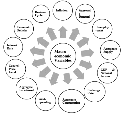
V. Unemployment
Unemployment occurs when individuals who are willing and able to work cannot find suitable employment. It is measured through the unemployment rate, which calculates the percentage of the labor force that is actively seeking jobs but remains unemployed. A high unemployment rate is an unfavorable economic indicator, as it signifies a large portion of the workforce is not engaged in productive activities, negatively impacting the economy.
VI. General Price Level
The general price level represents an index that reflects the overall prices of goods and services in an economy at the end of a specific period.
VII. Exchange Rate
The exchange rate plays a crucial role in international trade, enabling imports and exports between countries. It determines the value at which one country’s currency is exchanged for another’s. The exchange rate answers how many units of currency from country B can be obtained for one unit of currency from country A.
VIII. Interest Rate
Interest rate refers to the cost of borrowing money, determined by monetary authorities through various policies and market interventions. It is the amount a borrower pays to a lender for the use of funds. Different interest rates exist in an economy, and they vary based on the level of risk associated with lending.
IX. Government Spending
Government spending includes public sector expenditures on consumption, investment, and transfer payments. It represents the financial resources allocated to areas such as education, healthcare, transportation, social welfare, and defense. The government finances this spending through tax revenue and public borrowing.
X. GDP & National Income
Gross Domestic Product (GDP) is the total monetary value of all final goods and services produced within a country’s borders in an accounting year. It serves as a key indicator of economic health, with a rising GDP signifying increased production and economic growth. GDP is often considered a measure of national income, reflecting the purchasing power and financial well-being of a country’s population.
XI. Inflation
Inflation refers to a sustained increase in the general price level of goods and services over time, reducing the purchasing power of money. As demand for goods and services rises, their prices increase, leading to inflation. This means consumers must pay more to acquire the same goods and services. Inflation is a critical macroeconomic variable, as it is closely linked to factors like unemployment and economic growth. For instance, high unemployment can slow economic expansion, increasing the risk of inflation.
XII. Economic Policies
Economic policies serve as macroeconomic indicators and are broadly categorized into monetary and fiscal policies. Monetary policy focuses on regulating the money supply in the economy, while fiscal policy deals with government revenue and expenditures. These policies are formulated by the country’s central monetary authority and government to maintain economic stability.
XIII. Business Cycle
The business cycle refers to the fluctuations in a nation’s economic activity, particularly in GDP. It includes periods of expansion and contraction in production, trade, and overall economic activity. A recession occurs when there is a decline in aggregate output, while a prolonged and severe recession is known as a depression. The business cycle is a key macroeconomic indicator that helps analyze economic trends and stability.
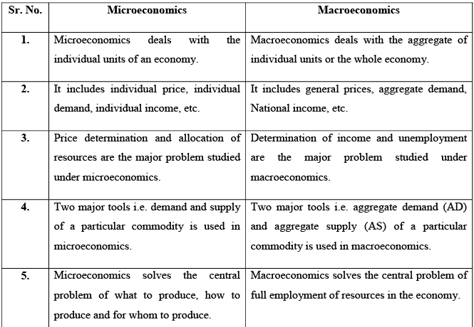
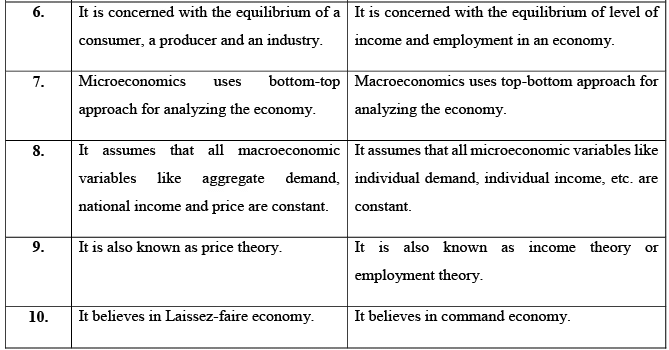
Difference between Macroeconomics and Microeconomics
Economics is a field of study that focuses on the production, consumption, and distribution of wealth. It is broadly divided into two branches: microeconomics and macroeconomics. Microeconomics examines the decision-making processes of individuals and businesses, whereas macroeconomics focuses on the policies and decisions of governments and large-scale economic entities. While the two branches are interdependent and cannot be fully understood in isolation, there are distinct differences between them. However, these differences are not absolute, as individual economic units influence the overall economy, and in turn, the overall economy affects its individual components.These are discussed as follows:
Table No. 1- Difference between microeconomics and macroeconomics

Interdependence of Macroeconomics and Microeconomics Theory
Microeconomics and macroeconomics are closely interconnected, as changes in one can directly influence the other. A small shift in microeconomic conditions can lead to broader macroeconomic effects, and vice versa. For example, an increase in aggregate demand can lead to higher individual demand for goods and services. This rise in demand may be triggered by a macroeconomic factor, such as a reduction in interest rates. Lower interest rates encourage borrowing, increasing the money supply and leading to higher consumer demand for products. As demand grows, industries require more labor, resulting in higher employment and wages. Increased wages, in turn, are supported by rising business profits, which stem from greater consumer demand. This cycle demonstrates how a macroeconomic change can directly impact microeconomic variables, highlighting the interdependence between the two economic theories.. Some other examples for explaining dependence of microeconomics on macroeconomics:
a. Payment made for means of production cannot be decided by an individual firm rather than these are dependent on the demand for means of production in the whole economy.
b. Sale of an individual firm is based on the purchasing power of consumer in the whole society.
c. For determining the demand for a product in an individual firm, it is necessary to study the demand of society, income and employment level in the economy.
Macroeconomics is not only influenced by microeconomics, but it is fundamentally built upon it. Since macroeconomics represents the sum of all microeconomic variables, it is essentially formed by the collective behavior of individuals, firms, households, and industries. For instance, national income is derived from the income of individuals and businesses, while macroeconomic indicators like aggregate consumption, investment, and savings are based on their microeconomic counterparts.
A clear example of this dependency can be seen when an economy directs all its resources toward producing capital goods. This shift can lead to a decline in total output, causing other sectors to suffer. As a result, the economy experiences a drop in overall income and employment, leading to an unequal distribution of wealth. Eventually, rising unemployment can push the economy into a state of depression. This illustrates how even a small change in a microeconomic variable can trigger significant shifts in macroeconomic conditions, reinforcing the interdependence between the two fields.
Some other examples for explaining dependence of macroeconomics on microeconomics:
a. National income is computed with the help of individual expenditure obtained from microeconomics.
b. Aggregate demand in the economy is computed with the help of demand of an individual firm.
According to Gardner Ackley, “Actually, the line between macroeconomics and micro economics theory cannot be precisely drawn. A true general theory of the economy would clearly embrace both. It would explain individual behavior, individual I outputs, incomes and prices and the sums or averages of individual results I would constitute the aggregates which macroeconomics is concerned”.
The same thing is suggested by Samuelson that “There is really no opposition between Micro and Macro Economics. Both are absolutely vital and you are only half-educated if you understand the one while being ignored or the other”. Thus, we can conclude that both micro and macro approaches are interrelated and interdependent on each other. Both approaches are helpful to analyze the economy.
Limitations of the Macroeconomics
Limitations of Aggregates
- Macroeconomics relies on aggregate data and behaviors, but what holds true for the economy as a whole may not be applicable to individuals. For example, an increase in overall savings can lead to economic depression if those savings are not invested. Similarly, if all bank depositors withdraw their money simultaneously, the financial system may collapse, affecting the entire economy.
Homogeneity Assumption in Aggregates
- Macroeconomic analysis assumes that all aggregates are homogenous, which may not always be the case. For instance, aggregate wages are calculated by combining wages from various occupations. If teachers' wages rise while clerks' wages decline, the overall wage level may appear unchanged, even though income distribution within occupations has shifted.
Misinterpretation of Aggregate Indicators
- Some macroeconomic indicators may not accurately reflect individual economic conditions. National income, for example, is measured as the total of all individual incomes. However, an increase in national income does not necessarily mean that all individuals have experienced income growth. Sometimes, the wealth of the rich increases while the lower-income groups see little or no improvement.
Challenges in Policy Application
- The application of macroeconomic theories to real-world scenarios can be problematic. Policies designed to achieve full employment in an economy may not be effective at the level of individual firms or industries. As a result, macroeconomic policies can sometimes provide misleading or impractical solutions.
Complexity in Measurement
- Calculating macroeconomic variables is a difficult and intricate process. Since macroeconomic data is derived from microeconomic statistics, it involves computing individual variables and then averaging them to create macroeconomic aggregates. This transformation is complex and can lead to errors, making the measurement process highly challenging.
Neglect of Individual Welfare
- Macroeconomics often prioritizes overall economic stability over individual well-being. For example, if national savings increase but come at the cost of reduced individual welfare, such a situation may not be beneficial for society. The focus on aggregates may overlook the impact on personal economic conditions.
Limited Applicability to Developing Nations
- Many macroeconomic models are designed primarily for developed economies and may not be suitable for developing countries. The unique economic challenges faced by developing nations often make it difficult for them to benefit from standard macroeconomic models.
Evolution of Macroeconomics
Macroeconomics did not develop overnight; rather, it evolved over many years through contributions from various economists, each presenting unique perspectives based on their analyses. The major schools of thought in macroeconomics are as follows:
1. Classical or Traditional School
Prominent economists such as Adam Smith, David Ricardo, and J.C.B. are associated with classical economic thought. They focused on studying economic issues from a broader, economy-wide perspective, advocating for macroeconomic analysis. Classical economists based their theories on Say’s Law of Markets and the flexibility of wages, interest rates, and prices. They argued that an economy naturally tends toward full employment, and any unemployment that occurs is only temporary. Their approach emphasized the self-regulating nature of macroeconomic variables.
2. Keynesian School of Thought
In 1936, John Maynard Keynes challenged classical theories in his book The General Theory of Employment, Interest, and Money. Keynes highlighted the limitations of classical thought, particularly opposing Say’s Law, which assumes that supply automatically creates its own demand. He argued that unemployment could persist for long periods due to insufficient aggregate demand. Keynesian economics emphasized the role of government intervention in boosting aggregate demand to reduce unemployment.
3. New-Classical or Monetarist School
Milton Friedman later opposed Keynesian ideas, introducing new-classical economic thought. This school rejected the notion that government intervention or fiscal policies could effectively reduce unemployment. Instead, it emphasized monetary policies, leading to its alternative name, monetarism. Friedman asserted that adjusting the money supply influences demand, which in turn helps achieve full employment in the economy.
4. Rational Expectations Theory and Further Developments
After 1960, economists such as Robert Lucas and John Muth introduced the Rational Expectations Theory, which further transformed macroeconomic thought. This theory suggested that individuals and businesses make decisions based on rational expectations about future economic conditions. Over time, several other developments and modifications have continued to shape macroeconomic theories.
Summary
Macroeconomics focuses on the study of aggregate economic variables and examines the economy as a whole. While both microeconomics and macroeconomics are interdependent, they differ in key aspects. Microeconomics primarily studies the decision-making processes of individuals and firms regarding scarce resources, whereas macroeconomics analyzes aggregated microeconomic variables at a broader level.
Macroeconomics is further categorized into three main areas:
Macro Static Analysis – Examines economic conditions at a specific point in time.
Macro Comparative Analysis – Compares different macroeconomic variables over time.
Macro Dynamic Analysis – Studies the changes and trends in macroeconomic variables over a period.
Several macroeconomic variables, such as national income, employment levels, and inflation, significantly impact the overall economy. The study of macroeconomics is as essential as microeconomics, given its broad scope, which includes theories of money, employment, and national income. Additionally, different schools of thought in macroeconomics have contributed to its evolution, reflecting the changing perspectives and approaches in economic analysis.
Despite certain limitations in its application, macroeconomics remains a crucial tool for understanding economic dynamics. It enables the measurement of key indicators such as national income, economic growth rate, and unemployment levels. Thus, macroeconomics plays a vital role in comprehending and managing the overall economy effectively.
|
59 videos|88 docs|29 tests
|
FAQs on Concepts of Macroeconomics (Part - 1) - Macroeconomics - Macro Economics - B Com
| 1. What is Macroeconomics? |  |
| 2. What are the main concepts of Macroeconomics? |  |
| 3. What is the difference between Macroeconomics and Microeconomics? |  |
| 4. What are the tools used in Macroeconomic analysis? |  |
| 5. Why is Macroeconomics important? |  |


