Differential Calculus | Quantitative Aptitude for CA Foundation PDF Download
INTRODUCTION
Differentiation is one of the most important fundamental operations in calculus. Its theory primarily depends on the idea of limit and continuity of function. To express the rate of change in any function we introduce concept of derivative which involves a very small change in the dependent variable with reference to a very small change in independent variable. Thus differentiation is the process of finding the derivative of a continuous function. It is defined as the limiting value of the ratio of the change (increment) in the function corresponding to a small change (increment) in the independent variable (argument) as the later tends to zero.
DERIVATIVE OR DIFFERENTIAL COEFFICIENT
Let y = f(x) be a function. If h (or Δx) be the small increment in x and the corresponding increment in y or f(x) be Δy = f(x+h) – f(x) then the derivative of f(x) is defined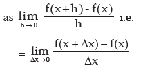
This is denoted as f’(x) or dy/ dx or  . The derivative of f(x) is also known as differential coefficient of f(x) with respect to x. This process of differentiation is called the first principle (or definition or abinitio) (Ab-initio)
Note: In the light of above discussion a function f (x) is said to differentiable at x = c if  exist which is called the differential coefficient of f(x) at x = c and is denoted
by 
We will now study this with an example.
Consider the function f(x) = x2.
By definition


Thus, derivative of f(x) exists for all values of x and equals 2x at any point x.
Examples of differentiations from the 1st principle
i) f(x) = c, c being a constant.
Since c is constant we may write f(x+h) = c.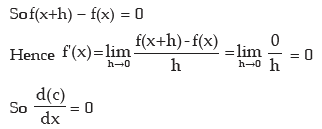
ii)
Now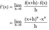


iii)
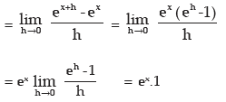

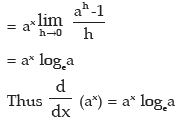
iv) Let f(x) = ax then f(x+h) = ax+h

v)
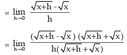
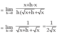

vi) f(x) = log x
∴ f(x + h) = log ( x + h)
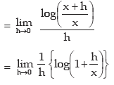
 i.e. h=tx and as h → 0, t → 0


SOME STANDARD RESULTS (FORMULAS)


Table: Few functions and their derivatives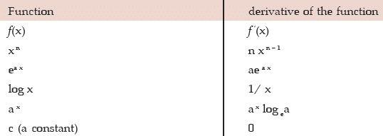
Table: Basic Laws for differentiation


It should be noted here even though in (ii), (iii), (iv) and (v) we have considered two functions f and g, it can be extended to more than two functions by taking two by two.
Example: Differentiate each of the following functions with respect to x:
(a) 3x2 + 5x –2
(b) ax + xa + aa
(d) exlog x
(e) 2x x5
(g) ex/ logx
(h) 2x.log x
Solution:
(a)
= 3 × 2x + 5.1 – 0 = 6x + 5
(b)

= ax log a + axa–1 + 0 = ax log a + axa–1.
(c)


(d) Let y = ex log x

(e)
(f)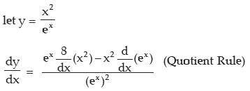

(g)
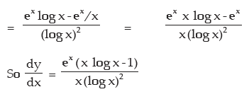
Let y = ex/logx
(h) Let h(x) = 2x.log x
The given function h(x) is appearing here as product of two functions
f (x) = 2x and g(x) = log x.

= 

(i)
Let  [Given function appears as the quotient of two functions]
f(x) = 2x and g(x) = 3x3 + 7


DERIVATIVE OF A FUNCTION OF FUNCTION
If y = f [h(x)]  where u = h(x)
Example: Differentiate log (1 + x2) wrt. x
Solution:
Let y = log (1 + x2) = log t when t = 1 + x2
This is an example of derivative of function of a function and the rule is called Chain Rule.
IMPLICIT FUNCTIONS
A function in the form f(x, y) = 0. For example x2y2 + 3xy + y = 0 where y cannot be directly defined as a function of x is called an implicit function of x. In case of implicit functions if y be a differentiable function of x, no attempt is required to express y as an explicit function of x for finding out  . In such case differentiation of both
sides with respect of x and substitution of  gives the result. Thereafter y1 may be obtained by solving the resulting equation.
Example: 
Solution: x2y2 + 3xy + y = 0
Differentiating with respect to x we see


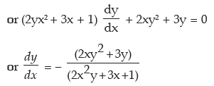
This is the procedure for differentiation of Implicit Function.
PARAMETRIC EQUATION
When both the variables x and y are expressed in terms of a parameter (a third variable), the involved equations are called parametric equations.
For the parametric equations x = f(t) and y = h(t) the differential coefficient dy/dx
is obtained by using
Example:
Solution: 

This is the procedure for differentiation of parametric functions.
LOGARITHMIC DIFFERENTIATION
The process of finding out derivative by taking logarithm in the first instance is called logarithmic differentiation. The procedure is convenient to adopt when the function to be differentiated involves a function in its power or when the function is the product of number of functions.
Example: Differentiate xx w.r.t. x
Solution: let y = xx
Taking logarithm,
log y = x log x
Differentiating with respect to x,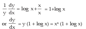
This procedure is called logarithmic differentiation.
SOME MORE EXAMPLES
1.
Solution: Taking logarithm, we may write 
Differentiating throughout we have

By cross–multiplication
Transposing 
(2)
Differentiate the following w.r.t. x:
Solution:


(b)


(3)
If xm yn = (x+y)m+n prove that 
Solution: xm yn = (x+y)m+n
Taking log on both sides
log xm yn = (m+n)log(x + y)
or m log x + n log y = ( m+n) log (x+y)
so
or
or
or
or
(4)
Solution: xy= ex–y
So y log x = (x – y) log e
or y log x = (x – y) ..............(a)
Differentiating w.r.t. x we get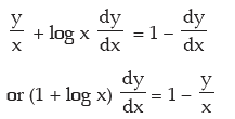
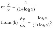
 , substituting x–y = log x, from (a) we have
BASIC IDEA ABOUT HIGHER ORDER DIFFERENTIATION
Since f(x) is a function of x it can be differentiated again
Thus
=12x2 + 30x + 4 is written as
  (read as d square y by dx square) and is called the second derivative of y with respect to x while dy/dx is called the first derivative. Again the second derivative here being a function of x can be differentiated again and
= f'''(x) = 24x +30.
Example: If y = aemx + be–mx prove that 
Solution:

GEOMETRIC INTERPRETATION OF THE DERIVATIVE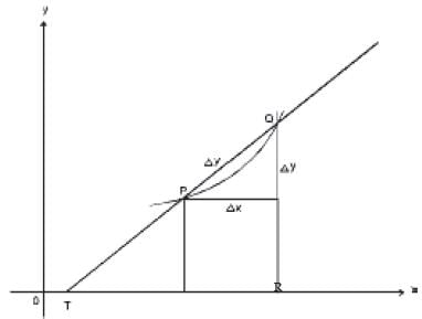
Let f(x) represent the curve in the fig. We take two adjacent pairs P and Q on the curve Let f(x) represent the curve in the fig. We take two adjacent points P and Q on the curve whose
coordinates are (x, y) and (x + Δx, y+Δy) respectively. The slope of the chord TPQ is given
by Δy/Δx when Δx →0, Q → P. TPQ becomes the tangent at P and 
The derivative of f(x) at a point x represents the slope (or sometime called the gradient of the curve) of the tangent to the curve y = f(x) at the point x. if  exists for a particular point say x =a and f(a) is finite we say the function is differentiable at x = a and continuous at that point.
Example: Find the gradient of the curve y = 3x2 – 5x + 4 at the point (1, 2).
Solution: y = 3x2 – 5x + 4

Thus the gradient of the curve at (1, 2) is 1.


Applications of Diffenential Calculus: In this chapter we have discussed the concept of differentiation. Differentiation helps us to find out the average rate of change in the dependent variable with respect to change in the independent variable. It makes differentiation to have applications. Various scientific formulae and results involves rate of change in price, change in demand with respect change in output, change in revenue obtained with respect change in price, change in demand with respect change in income, etc.
1) Rate of Change in Quantities: Let there two variables x and y such that y is a function of x. Differential coefficient dy/dx represents the rate of change of y with respect to x.
2) In other words, the expression, “the rate of Change of a function” means the derivative of the function.
3) We write f(x) in place of y and f’(x) in place of dy/dx
Cost Function: Total cost consists of two parts (i) Variable Cost (ii) Fixed Cost.
If C(X) denotes the cost producing x units of a product then C(x) = V(x) + F(x) , where V(x)
denotes the variable cost and F(x) is the fixed cost. Variable cost depends upon the number of units produced (i.e value of x) whereas fixed cost is independent of the level of output x. For example,

Marginal Cost: If C(x) the total cost producing x units then the increase in cost in producing one more unit is called marginal cost at an output level of x units and is given as dC/dx
Marginal Cost (MC) = Rate of change in cost C per unit change in Output at an output level of x units = dC/dx
To increase profits of a company may decide to increase its production. The question that concerns the management is how will the cost be affected by an increase in production.
Economists use the marginal cost to answer the question.
Example 1: The total cost function of a firm is where is the total cost and is outpout. A tax at the rate of ₹ 2 per unit of output is imposed and the producer adds it to his cost. If the market demand function is given by , where ₹ p is the price per unit of output, find the profit maximising output and price for maximum profit.
Solution:
After the imposition of tax of ₹ 2 per unit, the total new cost is
∴P(x) = R(x) - C(x)

For maximum total profit, and
P’(x) = 0 gives –x2 + 2500 = 0 ∴ x = ±50
Since output cannot be negative, we consider x = 50.
For x = 50, P”(x) = –2x = –2 x 50 = –100 < 0
Thus, the profit is maximum at x = 50.
Putting x = 50 in the demand function, the corresponding price is p=2530 – 5 × 50 = ₹ 2280
Example 2: The cost function of a company is given by:
where x denotes the output. Find the level of output at which:
(i) marginal cost is minimum
(ii) average cost is minimum
Solution:
M(x) = Marginal Cost = C(x) 
A(x) = Average Cost = 
(i) M(x) is maximum or minimum when M¢(x) = -16 + 2x = 0 or, x = 8.
Hence, marginal cost is minimum at x = 8.
(ii) A(x) is maximum or minimum when 

Hence, average cost is minimum at x = 12.
A(x) = Average Cost = 
= 100 - 96 + 48 = 52
1) Revenue Function: Revenue, R(x), gives the total money obtained (Total turnover) by
selling x units of a product. If x units are sold at ‘P per unit, then R(x) = P.X
Marginal Revenue: It is the rate of change I revenue per unit change in output. If R is the revenue and x is the output, then 
Profit function: Profit P(x), the difference of between total revenue R(x) and total Cost C (x). P(X)= R(x) – C(x)
Marginal Profit: It is rate of change in profit per unit change in output i.e dP/dx
Example 3: A computer software company wishes to start the production of floppy disks. It was observed that the company had to spend ₹2 lakhs for the technical informations. The cost of setting up the machine is ₹88,000 and the cost of producing each unit is ` 30, while each floppy could be sold at ₹45. Find:
(i) the total cost function for producing x floppies; and
(ii) the break-even point.
Solution:
a) Given, fixed cost = ₹2,00,000 +₹88,000 = ₹2,88,000.
(i) If C (x) be the total cost function for producing floppies, then C(x) = 30x + 2,88,000
(ii) The Revenue function R(x), for sales of x floppies is given by R(x) = 45x.
For break-even point, R(x) = C(x)
i.e., 45x = 30x + 2,88,000
i.e., 15x = 2,88,0000 ∴ x = 19,200, the break-even point
Example 4: A company decided to set up a small production plant for manufacturing electronic clocks. The total cost for initial set up (fixed cost) is ₹9 lakhs. The additional cost for producing each clock is ₹300. Each clock is sold at ₹750. During the first month, 1,500 clocks are produced and sold.
(i) What profit or loss the company incurs during the first month, when all the 1,500 clocks are sold ?
(ii) Determine the break-even point.
(b) Total cost of producing 20 items of a commodity is ₹205, while total cost of producing 10 items is ₹ 135. Assuming that the cost function is a linear function, find the cost function and marginal cost function.
Solution:
(a) The total cost function for manufacturing x Clocks is given by C(x) = Fixed cost + Variable cost to produce x Clocks = 9,00,000 + 300x.
The revenue function from the sale of x clocks in given by R(x) = 750 × x = 750x.
(i) Profit function,
P(x)= R(x) – C(x)
= 750x – (9,00,000 + 300x) = 450x – 9,00,000
∴ Profit, when all 1500 clocks are sold = P(1500) = 450 × 1500 – 9,00,000 = – ₹ 2,25,000
Thus, there is a loss of ₹ 2,25,000 when only 1500 clocks are sold.
(ii) At the break-even point, R(x) = C(x)
or, 9,00,000 + 300x = 750x
or, 450x = 9,00,000 ∴ x = 2,000
Hence, 2000 clocks have to be sold to achieve the break-even point.
b) Let cost function be
C(x) = ax + b, …………(i)
x being number of items and a, b being constants.
Given, C(x) = 205 for x = 20 and C(x) = 135 for x = 10.
Putting these values in (i),
205 = 20a+b …………(ii)
135 = 10a+b …………(iii)
(ii) – (iii) gives,
70 = 10a or, a = 7
From (iii), b = 135 – 10a = 135 – 70 = 65
∴ Required cost function is given by C(x) = 7x + 65
Marginal cost function, 
Marginal Propensity to Consume (MPC): The consumption function C = F(Y) expresses the relationship between the total consumption and total Income (Y), then the marginal propensity to consume is defined as the rate of Change consumption per unit change in Income i.e.,dC/dy. By consumption we mean expenditure incurred in on Consumption
Marginal Propensity to save (MPS): Saving, S is the difference between income, I and consumption, c, i.e . dS/dy
|
101 videos|209 docs|89 tests
|
FAQs on Differential Calculus - Quantitative Aptitude for CA Foundation
| 1. What is differential calculus? |  |
| 2. How is differential calculus used in real life? |  |
| 3. What is the difference between differential calculus and integral calculus? |  |
| 4. How do you find the derivative of a function? |  |
| 5. Can differential calculus be applied to non-linear functions? |  |


