Gradients and Related Operators - Civil Engineering (CE) PDF Download

Gradients and related operators
In this section, we consider scalar and vector-valued functions that assign a scalar and vector to each element in the subset of the set of position vectors for the points in 3D space. If x denotes the position vector of points in the 3D space, then  is a function that assigns a scalar Φ to each point in the 3D space of interest and Φ is called the scalar field. A few examples of scalar fields are temperature, density, energy. Similarly, the vector field û(x) assigns a vector to each point in the 3D space of interest. Displacement, velocity, acceleration are a few examples of vector fields.
Let  denote the region of the 3D space that is of interest, that is the set of position vectors of points that is of interest in the 3D space. Then a scalar field Φ, defined on a domain
  is said to be continuous if

where  denote the set of all position vectors of points in the 3D space a is a constant vector. The scalar field φ is said to be differential if there exist a vector field w such that
It can be shown that there is at most one vector field, w satisfying the above equation (proof omitted). This unique vector field w is called the gradient of Φ and denoted by grad(Φ).
The properties of continuity and differentiability are attributed to a vector field u and a tensor field T defined on a domain D, if they apply to the scalar field u·a and a · Tb ∀ a and b ∈  Given that the vector field u, is differentiable, the gradient of u denoted by
The divergence and the curl of a vector u denoted as div(u) and curl(u), are respectively scalar valued and vector valued and are defined by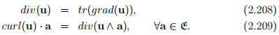
When the tensor field T is differentiable, its divergence denoted by div(T), is the vector field defined by
If grad(Φ) exist and is continuous, Φ is said to be continuously differentiable and this property extends to u and T if grad(u · a) and grad(a · Tb) exist and are continuous for all a, b ∈ 
An important identity: For a continuously differentiable vector field, u
div((grad(u))t ) = grad(div(u)). (2.211)
(Proof omitted)
Let Φ and u be some scalar and vector field respectively. Then, the Laplacian operator, denoted by ∆ (or by ∇2 ), is defined as
∆(Φ) = div(grad(Φ)), ∆(u) = div(grad(u)). (2.212)
The Hessian operator, denoted by ∇∇ is defined as
∇∇(Φ) = grad(grad(Φ)) (2.213)
If a vector field u is divergence free (i.e. div(u) = 0) then it is called solenoidal. It is called irrotational if curl(u) = o. It can be established that
curl(curl(u)) = grad(div(u)) − ∆(u). (2.214)
Consequently, if a vector field, u is both solenoidal and irrotational, then ∆(u) = o (follows from the above equation) and such a vector field is said to be harmonic. If a scalar field Φ satisfies ∆(Φ) = 0, then Φ is said to be harmonic.
Potential theorem: Let u be a smooth point field on an open or closed simply connected region R and let curl(u) = o. Then there is a continuously differentiable scalar field on R such that
u = grad(Φ) (2.215)
From the definition of grad (2.207), it can be seen that it is a linear operator. That is,
Consequently, all other operators div, ∆ are also linear operators.
Before concluding this section we collect a few identities that are useful subsequently. Here Φ, Ψ are scalar fields, u, v are vector fields and A is second order tensor field.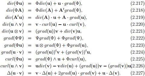
Till now, in this section we defined all the quantities in closed form but we require them in component form to perform the actual calculations. This would be the focus in the reminder of this section. In the following, let ei denote the Cartesian basis vectors and xi i = 1, 2, 3, the Cartesian coordinates.
Let Φ be differentiable scalar field, then it follows from equation (2.206), on replacing a by the base vectors ei in turn, that the partial derivatives  exist in D and that, moreover, wi = . Hence
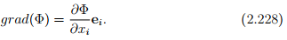
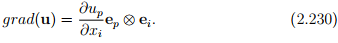
Let u be differentiable vector field in D and a some constant vector in E. Then, using (2.228) we compute
where ap and up are the Cartesian components of a and u respectively. Consequently, appealing to definition (2.207) we obtain
Then, according to the definition for divergence, (2.208)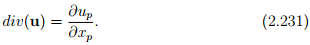
Next, we compute div(u ∧ a) to be
using (2.231). Comparing the above result with the definition of curl in (2.209) we infer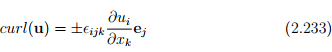
Finally, let T be a differentiable tensor field in  , then we compute
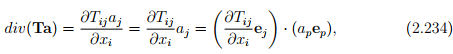
using equation (2.231). Then, we infer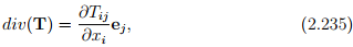
from the definition (2.210).
The component form for the other operators, namely Laplacian and Hessian can be obtained as respectively.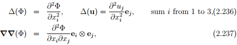
Above we obtained the components of the different operators in Cartesian coordinate system, we shall now proceed to obtain the same with respect to other coordinate systems. While using the method illustrated here we could obtain the components in any orthogonal curvilinear system, we choose the cylindrical polar coordinate system for illustration.
First, we outline a general procedure to find the basis vectors for a given orthogonal curvilinear coordinates. A differential vector dp in the 3D vector space is written as dp = dxiei relative to Cartesian coordinates. The same coordinate independent vector in orthogonal curvilinear coordinates is written as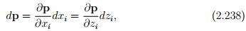
where zi denotes curvilinear coordinates. But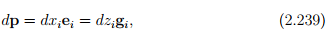
where gi is the basis vectors in the orthogonal curvilinear coordinates. Thus,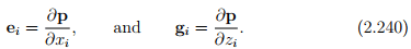
Comparing equations (2.239) and (2.240) we obtain the desired transformation relation between the bases to be: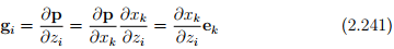
The basis gi so obtained will vary from point to point in the Euclidean space and will be orthogonal (by the choice of curvilinear coordinates) at each point but not orthonormal. Hence we define
and use these as the basis vectors for the orthogonal curvilinear coordinates.
Let (x, y, z) denote the coordinates of a typical point in Cartesian coordinate system and (r, θ, Z) the coordinates of a typical point in cylindrical polar coordinate system. Then, the coordinate transformation from cylindrical polar to Cartesian and vice versa is given by: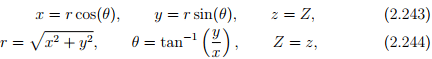
respectively. From these we compute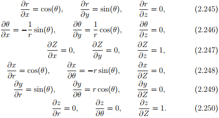
Consequently, the orthonormal cylindrical polar basis vectors (er, eθ, eZ) and Cartesian basis vectors (e1, e2, e3) are related through the equations
obtained using equation (2.242) along with a change in notation: ((ec)1, (ec )2,(ec )3) = (er, eθ, eZ).
Now, we can compute the components of grad(Φ) in cylindrical polar coordinates. Towards this, we obtain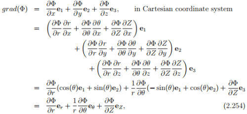
using the chain rule for differentiation.
To obtain the components of grad(u) one can follow the same procedure outlined above or can compute the same using the above result and the definition of grad (2.207) as detailed below: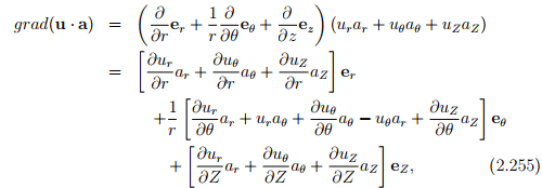
where we have used the following identities: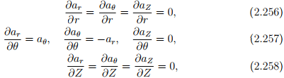
obtained by recognizing that only the Cartesian components of a are to be treated as constants and not the cylindrical polar components, ar = ax cos(θ) + ay sin(θ), aθ = −ax sin(θ) + ay cos(θ), aZ = az. From (2.255) and (2.207) the matrix components of grad(u) in cylindrical polar coordinates are written as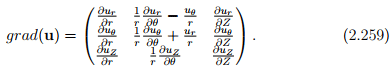
Using the techniques illustrated above the following identities can be established: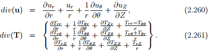
FAQs on Gradients and Related Operators - Civil Engineering (CE)
| 1. What is a gradient in image processing? |  |
| 2. How are gradients calculated in image processing? | |
| 3. What are the applications of gradients in image processing? | |
| 4. Can gradients be used for image smoothing or blurring? | |
| 5. How do gradients help in image segmentation? | |


Summary
,Sample Paper
,Gradients and Related Operators - Civil Engineering (CE)
,study material
,Important questions
,shortcuts and tricks
,mock tests for examination
,Gradients and Related Operators - Civil Engineering (CE)
,Free
,Semester Notes
,Exam
,ppt
,past year papers
,Viva Questions
,practice quizzes
,Extra Questions
,Previous Year Questions with Solutions
,Objective type Questions
,video lectures
,Gradients and Related Operators - Civil Engineering (CE)
,MCQs
;


Gradients and Related Operators Free PDF Download
Importance of Gradients and Related Operators
Gradients and Related Operators Notes
Gradients and Related Operators Civil Engineering (CE) Questions
Study Gradients and Related Operators on the App
|
© EduRev
|
Education Revolution
|


|


