Homogeneous Motions
Let us now understand what we mean when we say the motion to be homogeneous. Say, in the reference configuration, we have marked straight lines with different slopes on each of the three mutually perpendicular planes (material curves). Even, if only some of the line segments transform into curves the motion is inhomogeneous. Examples of such motions are plenty. A beam subjected to a pure bending moment6 is an example. Thus, we can show that for a homogeneous motion the matrix components of the deformation gradient, F with respect to a Cartesian basis can depend only on time and hence any homogeneous motion can be written in the form:
x = F(t)X + c(t), (3.116)
where c is some vector which depends on time, X and x are the position vectors of the same material particle in the reference and current configuration, respectively. Recognize that, in general, the matrix components of the deformation gradient, F with respect to a curvilinear basis (say cylindrical polar basis) need not be a constant for the deformation to be homogeneous nor would the deformation be homogeneous if the matrix components with respect to a curvilinear basis were to be a constant. For example, consider a deformation of the form:
r = R/g(Θ), θ = f(Θ), z = Z,
where
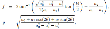
(R, Θ, Z) and (r, θ, z) are coordinates of the same material particle in cylindrical polar coordinates before and after deformation, ai’s are constants. A straightforward computation will show that the matrix components of deformation gradient tensor in cylindrical polar coordinates depends on Θ but when the same tensor is represented using Cartesian coordinates is independent of Θ.
| 6A long beam bends in such a way the plane sections normal to the axis of the beam remain plane. Hence, straight lines contained in planes perpendicular to the axis of the beam transform into straight lines. However, lines parallel to the axis of the beam transform into curves. |
Rigid body Motion
An example, of homogeneous motion is rigid body motion. Here apart from straight lines deforming into straight lines, the distance between any two points in the body remain the same. Let X1 and X2 be the position vectors of two material points in the reference configuration and let the position vector of the same material particle in the current configuration be denoted by x1 and x2, then, if the body undergoes rigid body motion:
| x1 − x2 |=| X1 − X2 | . (3.117)
Since, this motion is homogeneous
| x1 − x2 |=| F(X1 − X2) | . (3.118)
Combining equations (3.117) and (3.118) we obtain
(FtF − 1)(X1 − X2) = o. (3.119)
Since X1 ≠ X2 and (3.119) has to hold for any pair of material particles, i.e., X1 and X2 are some arbitrary but distinct vectors, we require that
FtF = 1, (3.120)
for a rigid body motion. Recalling the definition of an orthogonal tensor, (2.92) and comparing it with (3.120), we immediately recognize that for a rigid body motion, the deformation gradient has to be an orthogonal tensor. For example, consider, a motion given by
x = Q(t)[X − Xo] + c(t), (3.121)
where Q is an orthogonal tensor which is a function of time, Xo is a constant vector and c is a vector function of time.
Straight forward computation from the definition of the various quantities would show that the deformation gradient, F, the right and left CauchyGreen deformation tensors, C and B respectively, the Cauchy-Green strain tensor, E and the Almansi-Hamel strain tensor, e for this rigid body deformation are,
F = Q, C = 1, B = 1, E = 0, e = 0,
The Lagrangian displacement gradient, H and the Eulerian displacement gradient, h are:
H = Q − 1, h = 1 − Qt ,
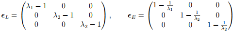
then, the Lagrangian linearized strain tensor, ∈L and the Eulerian linearized strain tensor, ∈E are evaluated to be,
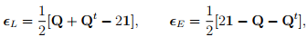
Observe that the given motion corresponds to rigid body rotation of the body about Xo and a translation. For this motion, we expect the strains to be zero because the length between two points do not change in a rigid body deformation. While the Cauchy-Green strain tensor and Almansi-Hamel strain tensor meets these requirements the linearized strain tensors don’t. However, recognize that these measures are valid only for cases when tr(HHt ) = tr(hht ) = tr(21 − Q − Qt ) << 1. That is to use linearized strain measures the rigid body rotation has to be small. Hence, linearized strain measures can be used only when the change in length is small and the angle of rotation of the line segment is small too.
Uniaxial or equi-biaxial motion
An uniaxial or equi-biaxial motion has the form:
x = λ1X, y = λ2Y, z = λ2Z, (3.122)
where λ1 and λ2 are functions of time and (X, Y, Z) denotes the Cartesian coordinates of a typical material particle in the reference configuration and (x, y, z) denote the Cartesian coordinates of the same material particle in the current configuration. If this motion is effected by the application of the force (traction) along just one direction (in this case along ex), then it is called uniaxial motion. On the other hand if the deformation is effected by the application of force along two directions(in this case along ey and ez), then it is called equi-biaxial motion.
For the assumed motion field (3.122), the deformation gradient, F, the right and left Cauchy-Green deformation tensors, C and B respectively, the Cauchy-Green strain tensor, E and the Almansi-Hamel strain tensor, e are
computed to be,
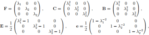
The Lagrangian displacement gradient, H and the Eulerian displacement gradient, h are:
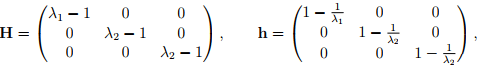
then, the Lagrangian linearized strain tensor, ∈L and the Eulerian linearized strain tensor, ∈E are evaluated to be,
Though the form of the Cauchy-Green, Almansi-Hamel, Lagrangian linearized and Eulerian linearized strain look different it can be easily verified that when λi is close to 1, numerically their values would also be close to each other.
Now, say a unit cube oriented in space such that B = {(X, Y, Z)|0 ≤ X ≤ 1, 0 ≤ Y ≤ 1, 0 ≤ Z ≤ 1} is subjected to a deformation of the form (3.122). Then, the deformed volume of the cube, v as given by (3.75) is v = det(F)  . Notice that the cube being of unit dimensions its original volume is 1. Similarly, the deformed surface area, a of the face whose normal coincides with ex in the reference configuration is computed from (3.74) as, a = det(F)
 and the deformed normal direction is found using Nanson’s formula (3.72) as, n = det(F)F−tex(1/a) = ex. The deformed length of a line element oriented along (ex + ey)/
  and of unit length is
  obtained by using (3.60). Similarly, the deformed angle between line segments oriented along ex and (ex + ey)/ is, αf = cos−1 (λ1/
  which is found using (3.66).
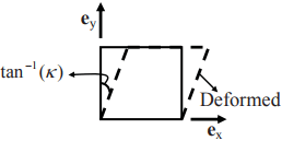
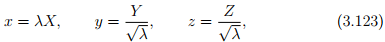
Figure 3.8: Schematic of simple shear deformation in the x-y plane
Isochoric motions
Motions in which the volume of a body does not change are called isochoric motions. Thus it follows from (3.75) that det(F) = 1 for these motions. In case of motions for which the magnitude of the components of the displacement gradient are small, then det(F) can be approximately computed as 1 + tr(∈) and thus for this deformation to be isochoric it suffices if tr(∈) = 0. Isochoric motion can be homogeneous or inhomogeneous. However, the examples that we shall consider here are homogeneous motions.
An isochoric uniaxial or equi-biaxial motion takes the form:
where λ is a function of time and as before (X, Y, Z) denotes the Cartesian coordinates of a typical material particle in the reference configuration and (x, y, z) denote the Cartesian coordinates of the same material particle in the current configuration. It is easy to check that det(F) for this deformation is 1.
A simple shear motion has the form:
x = X + κY, y = Y, z = Z, (3.124)
where κ is only a function of time. It is easy to verify that this motion is isochoric. In this case, the body is assumed to shear in the X − Y plane that is the angle between line segments initially oriented along the ex and ey direction change (see figure 3.8) but the angle between line segments initially oriented along ey and ez direction or ez and ex direction does not change.
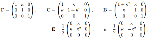
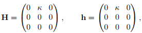
For the pure shear motion field (3.124), the deformation gradient, F, the right and left Cauchy-Green deformation tensors, C and B respectively, the Cauchy-Green strain tensor, E and the Almansi-Hamel strain tensor, e are computed to be,
The Lagrangian displacement gradient, H and the Eulerian displacement gradient, h are:
then, the Lagrangian linearized strain tensor,∈L and the Eulerian linearized strain tensor, ∈E are evaluated to be,
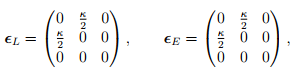
It can be seen from the above that while the Cauchy-Green and AlmansiHamel tells that the length of line segments along the ey direction would change apart from a change in angle of line segments oriented along the ex and ey directions, Lagrangian linearized and Eulerian linearized strain does not tell that the length of the line segments along ey changes. This is because, the change in length along the ey direction is of order κ2 , terms that we neglected to obtain linearized strain. Careful experiments on steel wires of circular cross section subjected to torsion7 shows axial elongation, akin to the development of the normal strain along ey direction. It is this observation that proved that linearized strain is an approximation of the actual strain.
7We shall see in chapter 8 that torsion of circular cross section is a pure shear deformation.
Now, say a unit cube oriented in space such that B = {(X, Y, Z)|0 ≤ X ≤ 1, 0 ≤ Y ≤ 1, 0 ≤ Z ≤ 1} is subjected to a deformation of the form (3.124). Then, the deformed volume of the cube, v as given by (3.75) is v = det(F) = 1. Similarly, the deformed surface area, a of the face whose normal coincides with ex in the reference configuration is computed from (3.74) as, a = det(F)  = 1 +κ2 and the deformed normal direction is found using Nanson’s formula (3.72) as, n = det(F)F−tex(1/a) = [ex − κey]/[1 + κ2 ]. The deformed length of a line element oriented along (ex + ey)/ and of unit length is p 1 + κ + κ 2/2 obtained by using (3.60). Similarly, the deformed angle between line segments oriented along ex and (ex + ey)/ is, αf = cos−1 ([1 + κ]/
 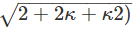 which is found using (3.66). In the above computations we have not assumed that the value of κ is small; if we do the final expressions would be much simpler.


