Illustrative Example - Boundary Value Problem: Formulation - Civil Engineering (CE) PDF Download

Illustrative example
Having formulated the boundary value problem and seen at techniques to solve it, in this section we illustrate the same by solving some standard boundary value problems.
Inflation of an annular cylinder In the first boundary value problem that is of interest, the body is in the form of an annular cylinder as shown in the figure 7.1. We use cylindrical polar coordinates to study this problem. Consequently, the body in the reference configuration is assumed to occupy a region in the Euclidean point space defined by, B = {(r, θ, z)|ri ≤ r ≤ ro, 0 ≤ θ ≤ 2π, 0 ≤ z ≤ L} that is the region between two coaxial right circular cylinders of radius riand ro respectively and of length L.
The boundary conditions that is of interest are also illustrated in figure 7.1. Thus, the cylinder is held fixed at constant length. Consequently, there is no axial displacement of the planes defined by z = 0 and z = L of the cylinder,
uz(r, θ, 0) = uz(r, θ, L) = 0, (7.58)
where uz represents the axial component of the displacement field. Then, the outer surface defined by r = ro, of the cylinder is traction free, i.e.,
 (7.59)
On the remaining surface, the inner surface defined by r = ri , of the cylinder only radial stress acts as shown in figure 7.1. Therefore,
 (7.60)
where pi is some positive constant. By virtue of the boundary conditions being independent of time and the constitutive relation is that of an elastic2 response, we are justified in assuming that the body is in static equilibrium under the action of boundary traction and hence a = o. Strictly, the traction boundary condition has to be applied on the deformed surface and not on the original surface. However, as discussed in section 7.2, we approximate the deformed surface with the original surface since they are close, in lieu of our assumptions that the magnitude of the displacement is small and that the magnitude of the components of the displacement gradient is also small.
To proceed further one has to decide whether to use displacement or stress as the basic unknown. Here we use displacement as the basic unknown. In general, one needs to solve the three partial differential equations involving the components of the displacement field, (7.22). Note by using (7.22) instead of (7.15), we have ignored the body forces and as per the discussion above we have assumed the body to be in static equilibrium.
Next, in order to avoid solving partial differential equations, appropriate assumptions are made for the displacement field so that the governing equation (7.22) reduces to a ordinary differential equation. This is possible because, for mixed boundary condition boundary value problems for bodies in static equilibrium and in the absence of body forces, it is shown in section 7.5.1 that there exist a unique solution for a body made up of a material that obeys isotropic Hooke’s law. In light of the boundary condition (7.58) we assume uz = 0. Further, we expect the cross section of the cylinder to deform as shown in the figure 7.2. That is we expect the circular cross section to remain circular but with a different radius and initially straight radial lines on the cross section to remain straight after deformation. Further we assume that there is no axial variation in the displacement field, that is any section along the axis of the cylinder deforms in the same fashion. These suggest that there is no circumferential component of the displacement field, i.e., uθ = 0 and that the radial component of the displacement field vary radially only. Thus,
u = ur(r)er. (7.61)
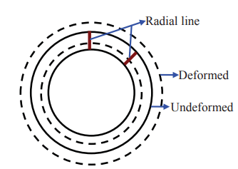
Figure 7.2: Schematic of deformation of the cross section of a right circular annular cylinder
Substituting equation (7.61) for displacement field in (7.22) and using equations (2.259), (2.260) and (2.261) we obtain
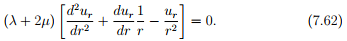
Since, (λ + 2µ) 6= 0, for equation (7.62) to hold we require
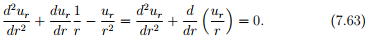
Solving the ordinary differential equation (7.63) we get
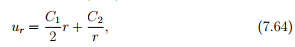
where C1 and C2 are integration constants to be found from the boundary conditions (7.59) and (7.60). Having found the unknown function in the displacement field (7.61), using (2.259) the cylindrical polar coordinate components of linearized strain can be computed as,
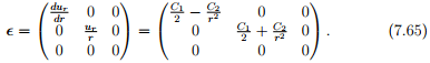
Substituting the above strain in the constitutive relation (7.2) the cylindrical polar coordinate components of the Cauchy stress is obtained as
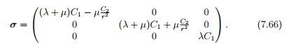
Recognizing that for the above state of stress, t(er) = [(λ+µ)C1 −µC2/r2 ]er, boundary conditions (7.59) and (7.60) yield
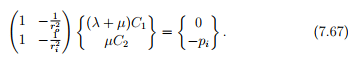
Solving the above equations we obtain:
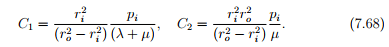
Substituting equation (7.68) in (7.66)
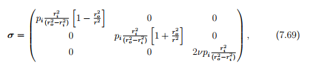
where we have used (6.79) to deduce that 2ν = λ/(λ + µ). Substituting equation (7.68) in (7.64),
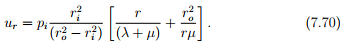
Figure 7.3 plots the variation of the radial (σrr) and hoop (σθθ) stresses with respect to r as given in equation (7.69) when ri = ro/2. It is also clear from equation (7.69) that the axial stresses do not vary across the cross section. When ri = ro/2, the constant axial stress value is 2piν/3. Thus, we find that due to inflation of the annular cylinder, tensile hoop stresses develop and the radial stresses are always compressive. The magnitude of the hoop stress is greater than radial stress. The magnitude of the axial stress is nearly one-tenth of the maximum hoop stress and it is tensile when ν > 0 and compressive when ν < 0 and is zero
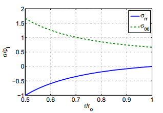
Figure 7.3: Plot of the radial (σrr) and hoop (σθθ) stresses given in equation (7.69) when ro = 1 and ri = ro/2.
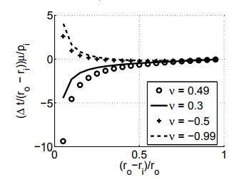

Figure 7.4: Plot of the variation in the ratio of change in thickness (∆t) of the cylinder to its original thickness (ro − ri) as a function of the thickness of the cylinder for various possible values of Poisson’s ratio, ν. µ is the shear modulus and pi is the radial component of the normal stress at the inner surface.
when ν = 0. Next, we physically explain this variation of the axial stresses with the Poisson’s ratio. The hoop stresses by virtue of being tensile in nature will cause a reduction in the axial length due to Poisson’s effect3 if the Poisson’s ratio, ν > 0 and increase in length if ν < 0 and no change if ν = 0. Similarly, the radial stress being compressive in nature will cause an increase in the axial length when ν > 0, decrease in axial length when ν < 0 and no change in axial length when ν = 0. However, the actual change in axial length would be a sum of both the change in length due to hoop and radial stress. Since, the hoop stress is more than the radial stress, if no axial force is applied, the axial length would reduce when ν > 0, will not change when ν = 0 and will increase when ν < 0. Thus, if the length is to remain unchanged, a tensile axial force has to be applied to counter the reduction in length when ν > 0 and a compressive axial force when ν < 0 and no axial force is required when ν = 0. It can be seen from the expression for axial stress in equation (7.69) that the expression for the axial stresses is consistent with the expectation that it be positive when ν > 0, negative when ν < 0 and zero when ν = 0. Now, we study the changes that occur to the thickness of the annular cylinder. Towards this, the ratio of change in thickness of the cylinder, ∆t to its original thickness is obtained as
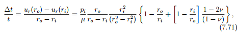
where we have used (6.80) to write Lam`e constants in terms of the Poisson’s ratio, ν and Young’s modulus E. Figure 7.4 plots the variation in the ratio of change in thickness of the cylinder to its original thickness as a function of the thickness of the cylinder for various possible values of Poisson’s ratio for a given radial component of the normal stress at the inner surface, pi . It can be seen from the figure that while the thickness decreases when ν ≥ 0, thickness increases when ν < 0 for thickness less than a critical value. By virtue of the radial component of the normal stress being compressive in nature one would expect a reduction in the thickness of the cylinder. However, the hoop stress being in tension, due to Poisson’s effect there would be reduction in thickness when ν > 0 and an increase when ν < 0. The actual change in the thickness is the sum of both the reduction due to radial stress and alteration
| Line elements on a plane whose normal coincides with the applied tensile stress shorten if ν > 0 and elongate if ν < 0. This effect is called as the Poisson’s effect. |
due to hoop stress. Hence, the thickness decreases when ν ≥ 0 and increases when ν < 0 for thickness less than a critical value.
Finally, we would like to show that due to inflation the inner as well as outer radius of the cylinder increases. Noting that the deformed inner radius of the cylinder is ri + u0(ri) and that of the deformed outer radius is ro + ur(ro), for these radius to increase we need to show that ur(ri) > 0 and ur(ro) > 0. Towards this, using equation (7.70) and (6.80) we obtain,
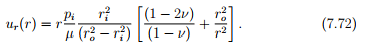
Recollecting from table 6.1, that the physically possible values for the Poisson’s ratio is: −1 < ν ≤ 0.5, it is straightforward to see that (1−2ν)/(1−ν) ≥ 0 for these possible range of values for ν. Also, it can be seen from table 6.1 that µ > 0. Further, by definition ro > ri and pi > 0. Therefore, ur(r) > 0 for any r, since each term in the expression for ur is positive. Hence, in particular ur(ri) > 0 and ur(ro) > 0 and hence the radius of the cylinder increases due to inflation, as one would expect.
Pressurized hole in an infinite medium
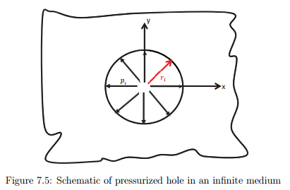
As a limiting case of the above solution, we would like to study the problem of a hole subjected to uniform radial component of the normal stress in an infinite medium as shown in figure 7.5. We continue to use cylindrical polar coordinates. Therefore the body in the reference configuration is assumed to occupy the region of the Euclidean point space defined by B = {(r, θ, z)|ri ≤ r < ∞, 0 ≤ θ ≤ 2π, −∞ < z < ∞}. The boundary conditions for this problem is essentially same as that in the inflation of an annular cylinder, except that now ro tends to ∞. For completeness the boundary conditions for the present problem is:
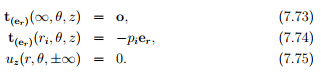
Hence, tending ro to ∞, in equations (7.69) and (7.70) we obtain the stress and displacement field for the present problem as,
Thus, we find that both the stress and the displacement tend to zero as r tends to ∞. This means that the effect of pressurized hole is not felt at a distance far away from the hole.
Having studied the problem of pressurized hole, in the following section we shall study the influence of the hole to uniaxial tensile load applied to the infinite medium with the hole.
Uniaxial tensile loading of a plate with a hole
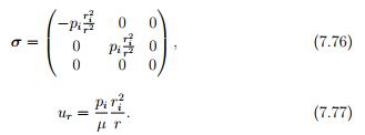
In the second boundary value problem that we study, the body is an infinite medium with a circular stress free hole subjected to a far field tension along the x−direction as shown in the figure 7.6. We envisage to solve this boundary value problem using the stress formulation. In particular we assume
Figure 7.6: Stress free hole in an infinite medium subjected to a uniform far field tension along x−direction
plane stress state and the body to be two dimensional and use cylindrical polar coordinates to study this problem. Thus, the body in the reference configuration is assumed to occupy a region in the Euclidean point space defined by B = {(r, θ)|a ≤ r < ∞, 0 ≤ θ ≤ 2π}, where a is a constant characterizing the size of the hole in the infinite medium. The boundary conditions that is of interest are
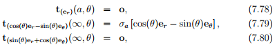
This boundary condition needs some explanation. The boundary condition (7.78) tells that the boundary of the hole is traction free i.e
σrr(a, θ) = 0, (7.81)
σrθ(a, θ) = 0. (7.82)
The second boundary condition (7.79) tells that the traction far away from the center of the hole, on a surface whose normal coincides with ex is σaex. Similarly, boundary condition (7.80) tells that a surface whose normal coincides with ey and is far away from the hole is traction free. In the equations (7.79) and (7.80), we have represented Cartesian basis ex and ey in cylindrical polar coordinate basis. From equations (7.79) and (7.80) we obtain,
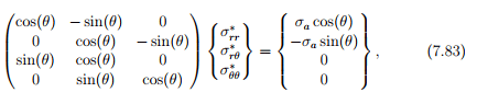
where  represents the value of the stress at (∞, θ). Of the four equations only 3 are independent. Picking any three equations and solving for the cylindrical polar components of the stress, we obtain
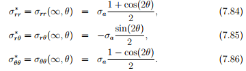
Thus, the boundary conditions translate into five conditions on the components of the stress given by equations, (7.81), (7.82), (7.84), (7.85) and (7.86).
Based on the observation that the far field stresses are a function of cos(2θ), we infer that the Airy’s stress function, φ also should contain cos(2θ) term. Then, since the solution at θ equal to 0 and 2π should be the same, the Airy’s stress function can depend on θ only through the trigonometric functions present in the general solution (7.57). We assume Airy’s stress function with only five constants from the general solution (7.57) as,

and examine whether the prescribed boundary conditions can be met. Consideration that the stress at ∞ be finite required dropping of the terms r2 ln(r) and r4 . The constant a01 does not enter the expressions for stress and examine whether the prescribed boundary conditions can be met. Consideration that the stress at ∞ be finite required dropping of the terms r2 ln(r) and r4 . The constant a01 does not enter the expressions for stress is computed using (7.53) to be
Now, the boundary conditions: (7.81), (7.82) and (7.84) yield:
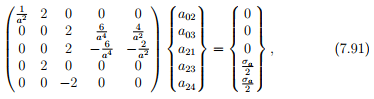
where we have equated the coefficients of cos(2θ), sin(2θ) and the constant to the values of the right hand side of these equations. It can be seen that the equations (7.85) and (7.86) yield the same last two equations in (7.91). Solving the linear equations (7.91) for aij ’s, we obtain
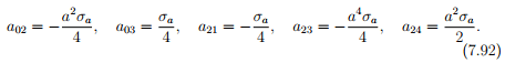
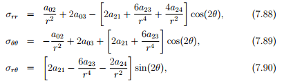
Since, we are able to meet the required boundary conditions with the assumed form of the Airy’s stress function, this is the required stress function. Substituting the constants (7.92) in the equations (7.88) through (7.90) we obtain
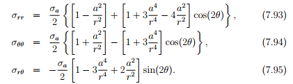
Having obtained the stress, we compute the strains from these stresses using the constitutive relation (7.54) as
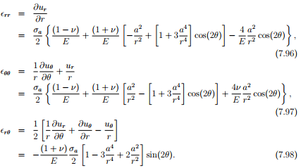
Integrating equation (7.96) we obtain
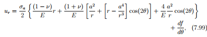
where f = ˆf(θ) is a function of θ. Substituting (7.99) in equation (7.97) and integrating we find

where g(r) is some function of r. Substituting equations (7.99) and (7.100) in equation (7.98) and simplifying we obtain
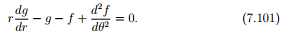
Since g is a function of only r and f only of θ, we require
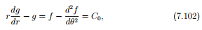
where C0 is a constant. Solving the linear ordinary differential equations (7.102) we obtain
g = C1r − C0, f = C0 + C2 exp(θ) + C3 exp(−θ), (7.103)
where Ci ’s are constants. To ensure that the tangential displacement of the ray θ = 0 and θ = 2π to be the same and there be no rigid body displacement we require that,
uθ(r, 0) = uθ(r, 2π) = 0. (7.104)
The condition (7.104) translates into requiring C1 = C2 = C3 = 0. Thus, the displacement field is computed to be,
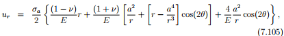
Thus, we have found the displacement and stress field and hence have solved this boundary value problem. We would like to find the maximum stress that occurs and its location for this boundary value problem.
First we begin with hoop stress, σθθ given in equation (7.94). Recollecting that the extremum value of a function could occur either at the boundary points or at points where the derivative of the function goes to zero, the extremum hoop stress could occur at a radial location, 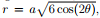 when cos(2θ) > 0 or at the boundary points, r = a and r tending to ∞. In figure 7.7 we plot the hoop stress as a function of r for various values of θ. As expected, the function is monotonically decreasing function of r when cos(2θ) < 0 and therefore the maximum value occurs at r = a for this case. When cos(2θ) > 0, the minimum occurs at r = a, then the maximum occurs when and then the stress decreases and asymptotically reaches the value of σa[1 − cos(2θ)]/2. Therefore, at r = a an extremum of the hoop stress occurs. The circumferential variation of the hoop stress at r = a is given by σa[1 − 2 cos(2θ)]. Hence, the maximum hoop stress occurs at r = a and θ = π/2 (or θ = 3π/2) and the value of the maximum hoop stress is 3σa. Thus, the stress concentration factor, defined as the ratio of the maximum stress in the structure to the far field stress is
Next, we study the circumferential shearing stress, σrθ given in equation (7.95). The extremum value of this stress occurs at a radial location r = a √ 3

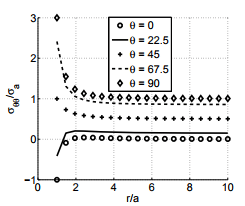
Figure 7.7: Variation of hoop stress, σθθ, with radial location, r for various orientation of the ray, θ when an infinite medium with a hole of radius a is subjected to a uniaxial tensile stress σa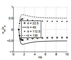
Figure 7.8: Variation of circumferential shearing stress, σrθ, with radial location, r for various orientation of the ray, θ when an infinite medium with a hole of radius a is subjected to a uniaxial tensile stress σa
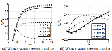
Figure 7.9: Variation of radial stress, σrr, with radial location, r for various orientation of the ray, θ when an infinite medium with a hole of radius a is subjected to a uniaxial tensile stress σa and the value of the circumferential shearing stress at this radial location is −2σa sin(2θ)/3. At the boundary points the circumferential shearing stress takes values 0 at r = a and −σa sin(2θ)/2. The variation of σrθ with the radial location, r and the orientation of the ray, θ is shown in figure 7.8. Thus, it can be seen that the absolute maximum value of the stress, σrθ occurs at r = a √ 3, θ = mπ/4, where m takes one of the values from the set {1, 3, 5, 7} and this maximum value is 2σa/3.
Finally, we examine the radial stress, σrr given in equation (7.93). An extremum value of this stress occurs at 
when4 0 ≤ θ ≤ π/6 or 2π/6 ≤ θ ≤ 4π/6 or 5π/6 ≤ θ ≤ 7π/6 or 8π/6 ≤ θ ≤ 10π/6 or 11π/6 ≤ θ ≤ 2π. This extremum value of the radial stress is −σa{11 cos(2θ)/9 + 1/9 + 5/[36 cos(2θ)]}/2. At the boundary the radial stresses takes the value 0 at r = a and σa[1 + cos(2θ)]/2 as r tends to ∞. Figure 7.9 portrays the variation of the radial stress with radial location, r for various orientations of the ray, θ. It can be seen from the figure that for certain orientations (say, θ = 90 degrees) the maximum value of the radial stress occurs at  and for some other 4The restriction on θ is obtained by the requirement that
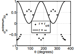
Figure 7.10: Variation of two extremum radial stress σrr at rcrit [given in equation (7.107)] and as r tends to ∞, with the orientation of the ray, θ when an infinite medium with a hole of radius a is subjected to a uniaxial tensile stress σa orientations (say, θ = 15 degrees) the maximum value occurs when r tends to ∞. To understand this, in figure 7.10 we plot the two extremum radial stresses - one at r = rcrit and the other value that occurs when r tends to ∞. It can be seen from the figure that when π/3 ≤ θ ≤ 2π/3 and 8π/3 ≤ θ ≤ 10π/3 the maximum radial stress occurs at rcrit and for all other values of θ it occurs as r tends to ∞. In any case the maximum value is always less than σa.
This concludes our illustration of the two techniques to solve boundary value problems in this chapter. However, in the remaining chapters we shall see employment of these techniques to solve more boundary value problems of interest in engineering.
FAQs on Illustrative Example - Boundary Value Problem: Formulation - Civil Engineering (CE)
| 1. What is a boundary value problem in mathematics? |  |
| 2. How is a boundary value problem different from an initial value problem? | |
| 3. What are some common examples of boundary value problems? | |
| 4. How can boundary value problems be solved? | |
| 5. Are boundary value problems only applicable in mathematics? | |


Illustrative Example - Boundary Value Problem: Formulation - Civil Engineering (CE)
,mock tests for examination
,past year papers
,ppt
,Semester Notes
,Objective type Questions
,practice quizzes
,Summary
,study material
,Illustrative Example - Boundary Value Problem: Formulation - Civil Engineering (CE)
,Extra Questions
,Free
,Viva Questions
,Important questions
,Sample Paper
,MCQs
,Exam
,Previous Year Questions with Solutions
,video lectures
,shortcuts and tricks
,Illustrative Example - Boundary Value Problem: Formulation - Civil Engineering (CE)
;


Illustrative Example - Boundary Value Problem: Formulation Free PDF Download
Importance of Illustrative Example - Boundary Value Problem: Formulation
Illustrative Example - Boundary Value Problem: Formulation Notes
Illustrative Example - Boundary Value Problem: Formulation Civil Engineering (CE) Questions
Study Illustrative Example - Boundary Value Problem: Formulation on the App
|
© EduRev
|
Education Revolution
|


|


within 7 days!