Additional Information about Integral Theorems for Civil Engineering (CE) Preparation
Integral Theorems Free PDF Download
The Integral Theorems is an invaluable resource that delves deep into the core of the Civil Engineering (CE) exam.
These study notes are curated by experts and cover all the essential topics and concepts, making your preparation more efficient and effective.
With the help of these notes, you can grasp complex subjects quickly, revise important points easily,
and reinforce your understanding of key concepts. The study notes are presented in a concise and easy-to-understand manner,
allowing you to optimize your learning process. Whether you're looking for best-recommended books, sample papers, study material,
or toppers' notes, this PDF has got you covered. Download the Integral Theorems now and kickstart your journey towards success in the Civil Engineering (CE) exam.
Importance of Integral Theorems
The importance of Integral Theorems cannot be overstated, especially for Civil Engineering (CE) aspirants.
This document holds the key to success in the Civil Engineering (CE) exam.
It offers a detailed understanding of the concept, providing invaluable insights into the topic.
By knowing the concepts well in advance, students can plan their preparation effectively.
Utilize this indispensable guide for a well-rounded preparation and achieve your desired results.
Integral Theorems Notes
Integral Theorems Notes offer in-depth insights into the specific topic to help you master it with ease.
This comprehensive document covers all aspects related to Integral Theorems.
It includes detailed information about the exam syllabus, recommended books, and study materials for a well-rounded preparation.
Practice papers and question papers enable you to assess your progress effectively.
Additionally, the paper analysis provides valuable tips for tackling the exam strategically.
Access to Toppers' notes gives you an edge in understanding complex concepts.
Whether you're a beginner or aiming for advanced proficiency, Integral Theorems Notes on EduRev are your ultimate resource for success.
Integral Theorems Civil Engineering (CE) Questions
The "Integral Theorems Civil Engineering (CE) Questions" guide is a valuable resource for all aspiring students preparing for the
Civil Engineering (CE) exam. It focuses on providing a wide range of practice questions to help students gauge
their understanding of the exam topics. These questions cover the entire syllabus, ensuring comprehensive preparation.
The guide includes previous years' question papers for students to familiarize themselves with the exam's format and difficulty level.
Additionally, it offers subject-specific question banks, allowing students to focus on weak areas and improve their performance.
Study Integral Theorems on the App
Students of Civil Engineering (CE) can study Integral Theorems alongwith tests & analysis from the EduRev app,
which will help them while preparing for their exam. Apart from the Integral Theorems,
students can also utilize the EduRev App for other study materials such as previous year question papers, syllabus, important questions, etc.
The EduRev App will make your learning easier as you can access it from anywhere you want.
The content of Integral Theorems is prepared as per the latest Civil Engineering (CE) syllabus.


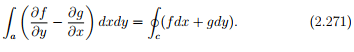

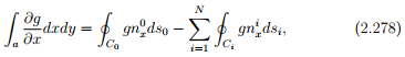
 defined over a planar simply connected domain,
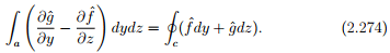
 reduces to
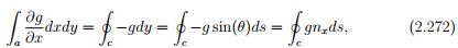
 yields
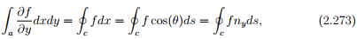