Isotropic Hooke’s law
Having established for isotropic materials if Cauchy stress is explicitly related to the deformation gradient, then this relationship would be of the form,
σ = f(F) = α01 + α1B + α2B−1 , (6.64)
where αi = âi(J1, J2, J3), called the material response functions and needs to be determined from experiments. Thus, restriction due to objectivity, has reduced the number of variables in the function from 9 to 3 and the number of unknown functions from 6 to 3. Next, let us see if we can further reduce the number of variables that the function depends upon or the number of functions themselves. Since, in an elastic process there is no dissipation of energy, this reduces the number of unknown functions to be determined to just one and thus Cauchy stress is given by ,
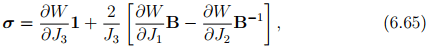
where W = Ŵ (J1, J2, J3), is called as the stored (or strain) energy per unit volume of the reference configuration. Notice that here the stored energy function is the only function that needs to be determined through experimentation.
In practice, the materials undergo a non-dissipative process only when the relative displacements are small, resulting in the components of the displacement gradient being small. Hence, it is of interest to see the implications of this approximation on a general representation for Cauchy stress (6.64). In chapter 3 (section (3.5.1), we saw that the deformation gradient is related to the Lagrangian and Eulerian displacement gradient as:
F = H + 1, F−1 = 1 − h. (6.66)
Hence, the left Cauchy-Green deformation tensor is given by
B = H + Ht + HHt + 1, B−1 = 1 − h − ht + hth. (6.67)
If tr(HHt ) << 1 and tr(hht ) << 1, then we could approximately calculate the left Cauchy-Green deformation tensor as
B ≈ H + Ht + 1, B−1 ≈ 1 − h − ht . (6.68)
We also saw in chapter 3 (section 3.8) that when tr(HHt ) << 1 and tr(hht ) << 1, H ≈ h. Therefore we need not distinguish between the Lagrangian and Eulerian linearized strain. By virtue of these approximations the expressions in equation (6.68) can be written as:
B ≈ 2∈ + 1, B −1 ≈ 1 − 2∈, (6.69)
where ∈ denotes the (Lagrangian or Eulerian) linearized strain tensor. Consequently, the invariants are calculated approximately as14
J1 ≈ 3 + 2tr(∈), J2 ≈ 3 − 2tr(∈), J3 ≈ 1 + tr(∈). (6.70)
Substituting (6.69) in a general representation for stress in a isotropic material, (6.64) we obtain
σ = α l 01 + α l 1 ∈. (6.71)
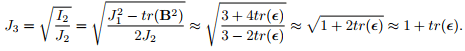
14 The last expression is obtained by substituting (6.69) in J3 =  and using Taylor’s series expansion about tr(∈) = 0, to obtain and using Taylor’s series expansion about tr(∈) = 0, to obtain
 |
where

are functions of tr(∈) by virtue of (6.70). It is necessary that  should be a linear function of tr(∈) and
  a constant; because we neglected the higher order terms of ∈ to obtain the above expression. Consequently, the expression for Cauchy stress (6.71) simplifies to,
σ = tr(∈)λ1 + 2µ∈, (6.73)
where λ and µ are Lam`e constants and these constants alone need to be determined from experiments. The relation (6.73) is called the Hooke’s law for isotropic materials.
Since, the relation between the Cauchy stress and linearized strain is linear we can invert the constitutive relation (6.73) and write the linearized strain in terms of the stress as,
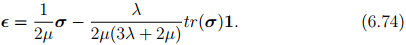
Taking trace on both sides of equation (6.73) we obtain,
tr(σ) = tr(∈)[3λ + 2µ], (6.75)
on noting that tr(·) is a linear operator and that tr(1) = 3. Thus, equation (6.74) is obtained by rearranging equation (6.73) and using equation (6.75). Lam`e constants while allows one to write the constitutive relations succinctly, their physical meaning and the methodology for their experimental determination is not obvious. Hence, we define various material parameters, such as Young’s modulus, shear modulus, bulk modulus, Poisson’s ratio, which have a physical meaning and is easy to determine experimentally.
Before proceeding further, a few comments on the Hooke’s law has to be made. From the derivation, it is clear that (6.73) is an approximation to the correct and more general (6.64). Consequently, Hooke’s law does not have some of the characteristics one would expect a robust constitutive relation to possess. The first drawback is that contrary to the observations rigid body rotations induces stresses in the body. To see how this happens, recall from chapter 3 (section 3.10.1) that linearized strain is not zero when the body is subjected to rigid body rotations. Since, strain is not zero, it follows from (6.73) that stress would be present. The second drawback is that the
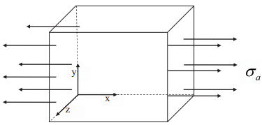
Figure 6.3: Uniaxial loading of a cuboid
constitutive relation (6.73) does not by itself satisfy the restriction due to objectivity. In fact it is not even Galilean invariant. Given that, due to equivalent placement of the body the displacement gradient transforms as given in equation (6.19) and Cauchy stress transforms as given in equation (6.25), it is evident that the restriction due to non-uniqueness of placers is not met. Despite these drawbacks, it is useful and gives good engineering estimates of the stresses and displacements under applied loads in certain classes of bodies.


