Lecture 2 - Introduction to Digital Control | 6 Months Preparation for GATE Electrical - Electrical Engineering (EE) PDF Download

Lecture 2 - Introduction to Digital Control, Control Systems
1 Discrete time system representations
As mentioned in the previous lecture, discrete time systems are represented by difference equations. We will focus on LTI systems unless mentioned otherwise.
1.1 Approximation for numerical differentiation
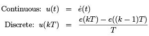
1. Using backward difference
(a) First order
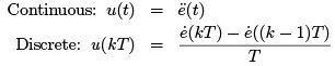
(b) Second order
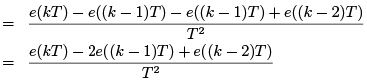
2. Using forward difference
(a) First order
(b) Second order
1.2 Approximation for numerical integration
The numerical integration technique depends on the approximation of the instantaneous continuous time signal. We will describe the process of backward rectangular integration technique.
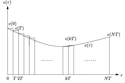
Figure 1: Concept behind Numerical Integration
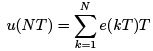
As shown in Figure 1, the integral function can be approximated by a number of rectangular pulses and the area under the curve can be represented by summation of the areas of all the small rectangles. Thus,
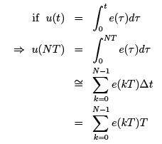
where k = 0, 1, 2, · · · , N − 1, ∆t = T and N > 0. From the above expression,
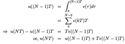
The above expression is a recursive formulation of backward rectangular integration where the expression of a signal at a given time explicitly contains the past values of the signal. Use of this recursive equation to evaluate the present value of u(N T ) requires to retain only the immediate past sampled value e((N − 1)T ) and the immediate past value of the integral u((N − 1)T ), thus saving the storage space requirement.
In forward rectangular integration, we start approximating the curve from top right corner.
Thus the approximation is
The recursive relation of the forward rectangular integration is:
u(N T ) = u((N − 1)T ) + T e(N T )
Polygonal or trapezoidal integration is another numerical integration technique where the total area is divided into a number of trapezoids and expressed as the sum of areas of individual trapezoids.
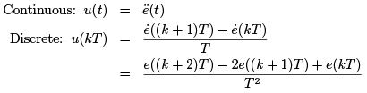
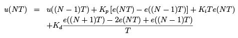
Example 1: Consider the following continuous time expression of a PID controller:
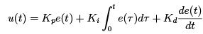
where u(t) is the controller output and e(t) is the input to the controller. Considering t = N T , find out the recursive discrete time formulation of u(N T ) by approximating the derivative by backward difference and integral by backward rectangular integration technique.
Solution: u(N T ) can be approximated as

Similarly u((N − 1)T ) can be written as
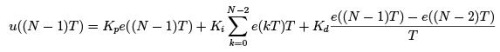
Subtracting u((N − 1)T ) from u(N T ),

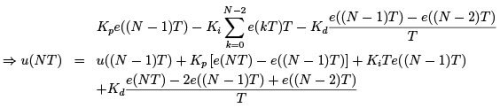
which is the required recursive relation.
Similarly, if we use forward difference and forward rectangular integration, we would get the recursive relation as
1.3 Difference Equation Representation
The general linear difference equation of an nth order causal LTI SISO system is:
y((k + n)T ) + a1y((k + n − 1)T ) + a2y ((k + n − 2)T ) + · · · + any (kT )
= b0u((k + m)T ) + b1u ((k + m − 1)T ) + .... + bmu (kT )
where y is the output of the system and u is the input to the system and m ≤ n. This inequality is required to avoid anticipatory or non-causal model.
Example 2: If you express the recursive relation for PID control in general difference equation form, is the system causal?
Solution: The output of the PID controller is u and the input is e. When approximated with forward difference and forward rectangular integration, u(N T ) is found as:
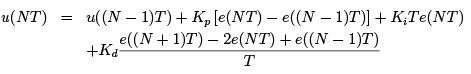
By putting N = k + 1 and comparing with general difference equation, we can say n = 1 whereas m = 2. Thus the system is non-causal. However, when the approximation uses backward difference and backward rectangular integration, the approximated model becomes causal.
|
675 videos|1379 docs|882 tests
|
FAQs on Lecture 2 - Introduction to Digital Control - 6 Months Preparation for GATE Electrical - Electrical Engineering (EE)
| 1. What is digital control? |  |
| 2. How does digital control differ from analog control? | |
| 3. What are the advantages of digital control? | |
| 4. Are there any disadvantages to digital control? | |
| 5. What are some applications of digital control? | |


Sample Paper
,Extra Questions
,Lecture 2 - Introduction to Digital Control | 6 Months Preparation for GATE Electrical - Electrical Engineering (EE)
,ppt
,past year papers
,mock tests for examination
,Important questions
,Lecture 2 - Introduction to Digital Control | 6 Months Preparation for GATE Electrical - Electrical Engineering (EE)
,Previous Year Questions with Solutions
,Summary
,Viva Questions
,Exam
,Lecture 2 - Introduction to Digital Control | 6 Months Preparation for GATE Electrical - Electrical Engineering (EE)
,Semester Notes
,Objective type Questions
,video lectures
,practice quizzes
,MCQs
,study material
,Free
,shortcuts and tricks
;


Lecture 2 - Introduction to Digital Control Free PDF Download
Importance of Lecture 2 - Introduction to Digital Control
Lecture 2 - Introduction to Digital Control Notes
Lecture 2 - Introduction to Digital Control Electrical Engineering (EE) Questions
Study Lecture 2 - Introduction to Digital Control on the App
|
© EduRev
|
Education Revolution
|


|


