Lecture 33 - Set Point Tracking | 6 Months Preparation for GATE Electrical - Electrical Engineering (EE) PDF Download

Lecture 33 - Set Point Tracking, Control Systems
1 Set Point Tracking
We discussed in the last lecture that a state feedback design can be done to place poles such that the system is stable. However, the tracking is not guaranteed.
1.1 Feed Forward Gain Design
Consider the state space model
x(k + 1) = Ax(k) + Bu(k)
y(k) = C x(k)
A control law is selected
u(k) = −K x(k) + N r(k)
as shown in figure 1 so that output can track any step reference command signal r. The closed loop dynamics of this configuration becomes
x(k + 1) = (A − BK )x(k) + BN r(k)
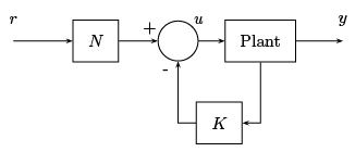
Figure 1: State feedback controller with feed forward gain for set point tracking
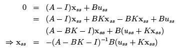
At steady state, say x = xss, y = C xss = r and u = uss.
Since the states or the output do not change with time in steady state, we can write
xss = Axss + Buss
Let us assume

Thus in shifted domain,
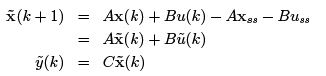
If we design a stable control  = −
= −  in the shifted domain, it will drive the state variables in shifted domain to 0.
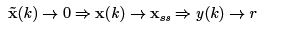
The problem of tracking is thus converted into a simple regulator problem.
We know that xss = Axss + Buss. Thus
 .
.
Now,
C xss = −C (A − BK − I )−1B(uss + K xss) = r
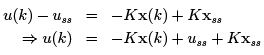
Thus the possible solution for N is uss + K xss = N r where
N−1 = −C (A − BK − I )−1B
and the control input is
u(k) = −K x(k) + N r
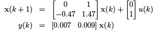
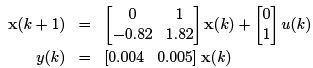
Example 1: Consider the following system
 .
.
Design a state feedback controller such that the output follows a step input with the desired closed loop poles at 0.5 and 0.6.
Solution: Desired characteristic equation:
z2 − 1.1z + 0.3 = 0
Open loop characteristic equation:
z2 − 1.47z + 0.47 = 0
The controller can be designed using the following expression u(k) = −K x(k) + N r
Since the system is in controllable canonical form, where the controllability matrix is UC =  .(non singular), the state feedback gain can be straight away designed as
K = [0.3 − 0.47 − 1.1 + 1.47] = [−0.17 0.37]
N can be designed as
N−1 = −C (A − BK − I )−1B = 0.08
Thus
u(k) = −[−0.17 0.37] x(k) + 12.5 r
1.2 State Feedback with Integral Control
Calculation of feed forward gain requires exact knowledge of the system parameters. Change in parameters will effect the steady state error.
In this scheme we feedback the states as well as the integral of the output error which will eventually make the actual output follow the desired one.
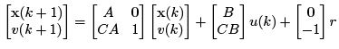
One way to introduce the integrator is to augment the integral state v with the plant state vector x.
v integrates the difference between the output y(k) and reference r. By using backward rectangular integration, it can be defined as
v(k) = v(k − 1) + y(k) − r
Thus
v(k + 1) = v(k) + y(k + 1) − r
= v(k) + C [Ax(k) + Bu(k)] − r
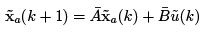
If we augment the above with the state equation,
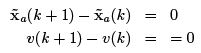
Since r is constant, if the system is stable, then x(k + 1) = x(k) and v(k + 1) = v(k) in the steady state. So, in steady state,
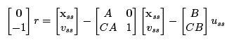
Let us define  . This implies
where 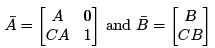
The design problem is now converted to a standard regulation problem. We need to design
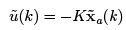
where K = [Kp Ki], Ki is the integral gain. Now,
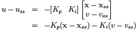
The steady state terms in the above expression must balance, which implies u(k) = −Kpx(k) − Kiv(k)
At steady state,
We can write from the above expression y(k) − r = 0 at steady state. In other words, y(k) follows r at steady state. The block diagram of state feedback with integral control is shown in Figure 2.
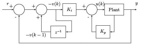
Figure 2: State feedback controller with integral control for set point tracking
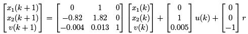
Example: Consider the problem of digital control of the following plant
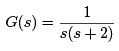
for a sampling period T = 0.1 sec using a state feedback with integral control such that the plant output follows a step input. The closed loop continuous poles of the system must be located at −1 ± j and −5 respectively.
Solution:
Discretization of the plant model gives
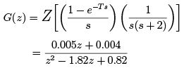
The discrete state space model of the plant is:
Augmenting the plant state vector with the integral state v(k), defined by v(k) = v(k − 1) + y(k) − r
we obtain
In terms of the state variables representing deviations from the steady state,
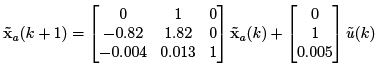
where  can be designed for the desired pole locations, 0.9 ± 0.1j and 0.6 (in discrete domain) using Ackermann’s formula, as,

Thus
u(k) = −[−0.328 0.416] x(k) − 0.889 v(k)
|
675 videos|1374 docs|882 tests
|
FAQs on Lecture 33 - Set Point Tracking - 6 Months Preparation for GATE Electrical - Electrical Engineering (EE)
| 1. What is set point tracking in control systems? |  |
| 2. Why is set point tracking important in control systems? | |
| 3. What are some challenges in achieving accurate set point tracking? | |
| 4. How can set point tracking be improved in control systems? | |
| 5. What are some applications of set point tracking in real-world systems? | |


ppt
,past year papers
,MCQs
,Lecture 33 - Set Point Tracking | 6 Months Preparation for GATE Electrical - Electrical Engineering (EE)
,Exam
,mock tests for examination
,Previous Year Questions with Solutions
,Lecture 33 - Set Point Tracking | 6 Months Preparation for GATE Electrical - Electrical Engineering (EE)
,video lectures
,shortcuts and tricks
,Summary
,Semester Notes
,practice quizzes
,Objective type Questions
,Viva Questions
,Extra Questions
,Important questions
,Free
,Sample Paper
,study material
,Lecture 33 - Set Point Tracking | 6 Months Preparation for GATE Electrical - Electrical Engineering (EE)
;


Lecture 33 - Set Point Tracking Free PDF Download
Importance of Lecture 33 - Set Point Tracking
Lecture 33 - Set Point Tracking Notes
Lecture 33 - Set Point Tracking Electrical Engineering (EE) Questions
Study Lecture 33 - Set Point Tracking on the App
|
© EduRev
|
Education Revolution
|


|


