Lecture 8 - Modeling Discrete Time Systems by Pulse Transfer Function | 6 Months Preparation for GATE Electrical - Electrical Engineering (EE) PDF Download

Lecture 8 - Modeling discrete-time systems by pulse transfer function, Control Systems
1 Pulse Transfer Functions of Closed Loop Systems
We know that various advantages of feedback make most of the control systems closed loop nature. A simple single loop system with a sampler in the forward path is shown in Figure 1.
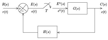
Figure 1: Block diagram of a closed loop system with a sampler in the forward path The ob jective is to establish the input-output relationship. For the above system, the output of the sampler is regarded as an input to the system. The input to the sampler is regarded as another output. Thus the input-output relations can be formulated as
E (s) = R(s) − G(s)H (s)E ∗(s) (1)
C (s) = G(s)E ∗(s) (2)
Taking pulse transform on both sides of (1),
E∗(s) = R∗(s) − GH ∗(s)E ∗(s) (3)
where
GH ∗(s) = [G(s)H (s)]∗
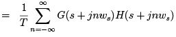
We can write from equation (3),
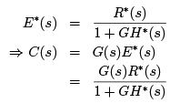
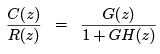
Taking pulse transformation on both sides of (2)
where GH (z) = Z [G(s)H (s)].
Now, if we place the sampler in the feedback path, the block diagram will look like the Figure 2.
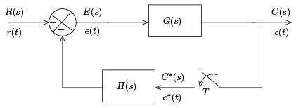
Figure 2: Block diagram of a closed loop system with a sampler in the feedback path
The corresponding input output relations can be written as:
E(s) = R(s) − H (S )C ∗(s) (4)
C(s) = G(s)E (s) = G(s)R(s) − G(s)H (s)C ∗(s) (5)
Taking pulse transformation of equations (4) and (5)
E∗(s) = R∗(s) − H ∗(s)C ∗(s)
C∗(s) = GR∗(s) − GH ∗(s)C ∗(s)
where, GR∗(s) = [G(s)R(s)]∗
GH ∗(s) = [G(s)H (s)]∗
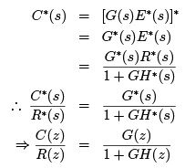
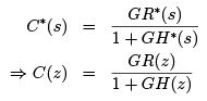
C∗(s) can be written as
We can no longer define the input output transfer function of this system by either 
 Since the input r(t) is not sampled, the sampled signal r∗(t) does not exist. The continuous-data output C (s) can be expressed in terms of input as.
C (s) = G(s)R(s) 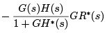
1.1 Characteristics Equation
Characteristics equation plays an important role in the study of linear systems. As said earlier, an nth order LTI discrete data system can be represented by an nth order difference equation,
c(k + n) + an−1c(k + n − 1) + an−2c(k + n − 2) + ... + a1c(k + 1) + a0c(k)
= bmr(k + m) + bm−1r(k + m − 1) + ... + b0r(k)
where r(k) and c(k) denote input and output sequences respectively. The input output relation can be obtained by taking Z-transformation on both sides, with zero initial conditions, as
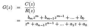 (6)
(6)
The characteristics equation is obtained by equating the denominator of G(z) to 0, as
zn + an−1zn−1 + ... + a1z + a0 = 0
Example
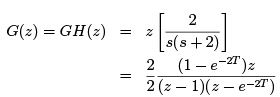
Consider the forward path transfer function as G(s) =  and the feedback transfer function as 1. If the sampler is placed in the forward path, find out the characteristics equation of the overall system for a sampling period T = 0.1 sec.
Solution:
Since the feedback transfer function is 1,
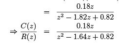
So, the characteristics equation of the system is z 2 − 1.64z + 0.82 = 0.
1.2 Causality and Physical Realizability
- In a causal system, the output does not precede the input. In other words, in a causal system, the output depends only on the past and present inputs, not on the future ones.
- The transfer function of a causal system is physically realizable, i.e., the system can be realized by using physical elements.
- For a causal discrete data system, the power series expansion of its transfer function must not contain any positive power in z . Positive power in z indicates prediction. Therefore, in the transfer function (6), n must be greater than or equal to m.
m = n ⇒ proper transfer function
m < n ⇒ strictly proper Transfer function
|
675 videos|1379 docs|882 tests
|
FAQs on Lecture 8 - Modeling Discrete Time Systems by Pulse Transfer Function - 6 Months Preparation for GATE Electrical - Electrical Engineering (EE)
| 1. What is a pulse transfer function? |  |
| 2. How is a pulse transfer function different from a transfer function? | |
| 3. How can I model a discrete time system using a pulse transfer function? | |
| 4. What are the advantages of using a pulse transfer function for modeling discrete time systems? | |
| 5. Can a pulse transfer function be used to model continuous time systems? | |


past year papers
,Semester Notes
,Exam
,study material
,video lectures
,practice quizzes
,Viva Questions
,Previous Year Questions with Solutions
,Lecture 8 - Modeling Discrete Time Systems by Pulse Transfer Function | 6 Months Preparation for GATE Electrical - Electrical Engineering (EE)
,Lecture 8 - Modeling Discrete Time Systems by Pulse Transfer Function | 6 Months Preparation for GATE Electrical - Electrical Engineering (EE)
,Sample Paper
,Objective type Questions
,Extra Questions
,Summary
,Lecture 8 - Modeling Discrete Time Systems by Pulse Transfer Function | 6 Months Preparation for GATE Electrical - Electrical Engineering (EE)
,Important questions
,Free
,mock tests for examination
,ppt
,MCQs
,shortcuts and tricks
;


Lecture 8 - Modeling Discrete Time Systems by Pulse Transfer Function Free PDF Download
Importance of Lecture 8 - Modeling Discrete Time Systems by Pulse Transfer Function
Lecture 8 - Modeling Discrete Time Systems by Pulse Transfer Function Notes
Lecture 8 - Modeling Discrete Time Systems by Pulse Transfer Function Electrical Engineering (EE) Questions
Study Lecture 8 - Modeling Discrete Time Systems by Pulse Transfer Function on the App
|
© EduRev
|
Education Revolution
|


|


