MS Excel | Cyber Olympiad for Class 9 PDF Download

Microsoft Excel is an electronic spreadsheet. Spreadsheets are made up of columns, rows and their intersections are called cells. It is used  to organize your data into rows and columns. You can also use it to perform mathematical calculations quickly.

Each cell of the spreadsheet may contain the following types of data:

• Text
• Numberical  data
• Formulae (mathematical equations that do all the work)

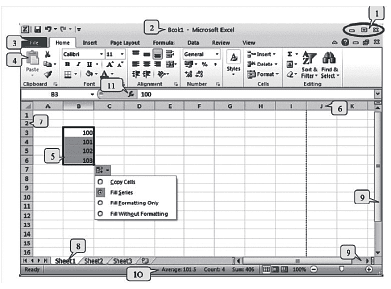
Microsoft Excel Interface

(i) These buttons are used for manipulation of Excel window such as minimize,  maximize, close window
(ii) Title Bar contains document’s name, extension (.xisx) and the program name.
(iii) A list of tabs found in excel window are

• File
• Home
• Insert
• Page layout
• Formulas
• Data
• Review
• View

(iv) Toolbars give you a variety of options to carry out different tasks. clicking on the downwind arrow of tool reveals a list of more options related to that tool. Tools that cannot be applied to a selected object are greyed out.
The tools that have dots, if pressed, lead to another sequence of commands Toolbars with tabs is called a Ribbon.
(v) Selected cells: before we enter a text, number or other data, we must first select a cell or cells.
(vi) Column titles (letters)
(vii) Row titles (numbers)
(viii) Sheets
(ix) Bars for horizontal and vertical navigation (sliders)
(x) Status bar: displays information about some special functions of Microsoft Excel.
(xi) Shows the space  bar for formulas

One of Excel’s most useful features is that it  allows users to create custom formulas to perform calculations on their data. Excel also contains built-in formulas called functions that make it easy to perform common calculations on data.

Formula Basics

Formulas in Microsoft Excel begin with an equal to sign. The equal to sign tells Excel that the succeeding characters will constitute a formula. If you don’t enter the equal to sign, Excel will treat your entry as text and the calculation will fail.
If you select a blank cell A1 and type =5+5, and press Enter, Excel will perform the calculation and produces a result of 10 in the cell A1.

Operations in Formulas
Following are different operations used in Formulas: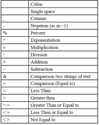
Functions and Formulas
MS Excel provides many formulas to perform several methodical calculations.  The organization of formulas is new to Excel 2010. In Excel 2007, to obtain all the formulas, you had to click on the AutoSum drop-down arrow and select More Functions. The same options that appeared in the More Functions dialog box now appear on the Formula Tab. Each formula is divided into relevant general topic categories. The categories are listed across the top of the Formula Tab group titled Function Library.

With the new Excel Formula Bar, the majority of all formulas you may need are at your fingertips.
For example: a Math professor is interested in determining which formula would be the best to convert radians to degrees. We will go to the Formula Tab, and select the Math and Trig downward arrow.
Tip: When you scroll the mouse over a formula Excel will have a small dialog box that explains the purpose of each formula.

How to Apply Basic Formulas

Adding Values in Rows or Columns
(i) Use the SUM function, which is a pre-written formula, to add all the values in a row or column:

• Click your mouse in the cell in which you wish your result to appear.
• Click the AutoSum button on the Home Tab or the Formulas Tab.
• Highlight the range of cells you wish to add.
• Press Enter.

(ii) To add some of the values in a column or row:

• Type an equal to sign, type SUM, then type an opening parenthesis.
• Type or select the cell references you want to add. A comma (,) separates individual arguments that tell the function what to calculate.
• Type a closing parenthesis, and then press ENTER.
  For example: =SUM(B2:B4, B6) and =SUM(B2, B5, B7)

Finding the Average, Maximum, or Minimum
Use the AVERAGE, MAX, OR MIN functions.

• Click your mouse in the cell in which you wish your result to appear.
• Click the arrow next to AutoSum on the Home Tab or the Formulas Tab.
• Click the Average, Max, or Min.
• Highlight the range of cells you wish to find the value for.
• Press Enter.

To see more functions, click More Functions on the AutoSum list to open the Insert Function dialog box or go to the Formulas Tab and click on the More Functions orange textbook icon.
Tip: You can also enter formulas and cell references by typing them in the formula bar after selecting a cell.

Select Ranges and Individual Cells

• As you start to write excel formulas, you may realize you want to use a range of cells or nonadjacent cells in your formula. A range of cells will include the value of every cell within the range specified (for example, the range A1:A4 includes the cells A1, A2, A3 & A4).
  Ranges of cells are identified with a colon.
• Non-adjacent cells can be listed in the formula by separating them with a comma rather than a colon. For example, =SUM(A2,A4) will add cells A2 and A4, but not A3.

Copying a Formula

(i) Using the Fill Handle
(a) Select the cell that contains the formula, then position the mouse pointer over the lower-right corner of the cell until the black cross (+) appears.
(b) Drag the fill handle over the cell or cells to which you want to copy the formula, then release the mouse button.

(ii) Using Traditional Copy and Paste

(a) Select the cell that contains the formula, and on the Edit menu, click Copy.

(b) Select the cell or cells that you want to copy the formula to.

• To copy the formula choose the Edit menu, click Paste.
• To copy the formula, only, on the Edit menu, click Paste Special, and then click Formulas.

Referencing Cells in Formulas
You can include or refer other cells in a formula. The result of the formula depends on the values in the refered cells and changes automatically when the values in the refered cells change. This is extremely powerful in what-if cases.
To see how this works, enter 10 in cell A1. Now select cell A2 and type =A1*2, and press ENTER. The value in cell A2 is 20. If you change the value in cell A1 from 10 to any value, the value in cell A2 will also change. Cell references are especially helpful when you create complex formulas, or conduct what-if analysis. (See the table below)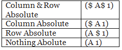

Pressing F4 repeatedly over a reference cell will allow you to switch between making the column, the row, or nothing ‘Absolute.’.

Adding,Subtracting, Multiplying and Divide
Type an equal to sign (=), use math operators, and then press ENTER.
=10+5 to add
=10-5 to subtract
=10*5 to multiply
=10/5 to divide
Formulas are visible in the formula bar
when you select a cell that contains a result. If the formula bar is not visible, on the Tools menu, click Options. Click the View tab, and select the Formula bar check box.

Understanding Error Values

#####: It shows that the column is not wide enough to display the content. Increase column width, shrink contents to fit the column, or apply a different number format.
#REF!: It means a cell reference is not valid. Cells may be deleted or pasted over.
#NAME?: It refers that you may have misspelled a function name.

Mathematical and Trigonometrical formulas functions

The PRODUCT function provides a quick way to multiply numbers in the Excel. The advantage of using this function becomes apparent when you have several numbers to multiply together. It is easier than creating long formula.

The syntax for the PRODUCT function is:
=PRODUCT( Number1, Number2, ... Number255 )
TIP: Up to 255 numbers can be entered into the function.

SUMIF Function
The SUMIF function is used to add up the values in cells in a selected range that meet certain criteria.

The syntax for the SUMIF function is:
= SUMIF (Range, Criteria, Sum Range)

• Range: Searches a group of cells within the given range
• Criteria: This determines whether the cell is to be counted or not.
• Sum Range: The data range that is summed if the first range meets the specified criteria. If this range is omitted, the first range is summed instead.

SUMIFS Function The SUMIFS function adds up the data in selected cells when specific criteria are met in two or more ranges of data.

The syntax for the SUMIFS function is:

=SUMIFS ( Sum_range, Criteria_range1, Criteria1, Criteria_range2, Criteria2, ...)

• Sum_range: the range of cells to be added.
• Criteria_range: the range of cells the function is to search.
• Criteria: this determines whether a cell in the Sum_range is to be counted or not.
• Note: Up to 127 range/criteria pairs can be entered into the function.

ROUND Function

The ROUND function is used to reduce a given value to a specific number of decimal places.

The syntax for the ROUND function is:

= ROUND ( Number, Num_digits )

• Number: it is the value to be rounded.
• Num_digits: the number of decimal places to reduce the above number to.

Logical Function
IF Function
The IF function, one of Excel’s logical functions, tests to see if a certain condition in a spreadsheet is true or false.

The syntax for the IF function is: =IF ( logical_ test, value_if_true, value_if_false )

• logical_test: a value or expression that is tested to see if it is true or false.
• value_if_true: the value that is displayed if logical_test is true.
• value_if_false: the value that is displayed if logical_test is false.

Lookup and Reference Functions

VLOOKUP Function
Excel’s VLOOKUP function, which stands for vertical lookup, is used to find specific information that has been stored in a spreadsheet table.
Note: The data in the table should be sorted in ascending order (alphabetically A to Z).

The syntax for the VLOOKUP function is: = VLOOKUP ( lookup_value , table_array , col_index_num ,range_lookup )

• lookup _value: The value you want to find in the first column of the table_array.
• table_array: This is the table of data that VLOOKUP searches to find the information you are looking for.
  The table_array must contain at least two columns of data. The first column contains the lookup_ values.
• col_index_num: The number of the column in the table_array that contains the data you want returned.
• range_lookup: A logical value (TRUE or FALSE only) that indicates whether you want VLOOKUP to find an exact or an approximate match to the lookup_value. Typing False will return exact matches only.

Date & Time Functions

NETWORKDAYS Function

The NETWORKDAYS function, can be used to count the number of working days between two dates - such as the start and end dates for a project. The function automatically removes weekends  from the total. Specific holidays can also be omitted.
The syntax for the NETWORKDAYS function is: = NETWORKDAYS ( Start_date , End_date , Holidays )

• Start_date: the start date of the chosen time period.
• End_date: the end date of the chosen time period.
• Holidays: can be used to exclude one or more dates from the total number of working days (optional).

NOW Function
The NOW function, is used to add the current time and date to a spreadsheet.
The syntax for the NOW function is: = NOW ( )
Note: The NOW function takes no arguments.

AutoSum Function
AVERAGE Function: The AVERAGE function, is used to find the average or arithmetic mean of a given list of arguments. The syntax for the AVERAGE function is:
= AVERAGE ( argument1, argument2, ... argument255 )
Argument1, argument 2, ... argument 255 can be numbers, named ranges, arrays, or cell references.
Tip: Up to 255 arguments can be entered.

MAX Function
The MAX function, is used to find the largest or maximum number in a given list of values or arguments. The syntax for the MAX function is:

=MAX( argument1, argument2, ..argument30 )
Argument1 ... argument 30: The arguments can be numbers, named ranges, arrays, or cell references. Up to 30 arguments can be entered.

MIN Function
The MIN function, is used to find the smallest or minimum value in a list of numbers or arguments. The syntax for the MIN function is:
= MIN ( argument1, argument2, ... argument30 )
Argument1 ...argument 30: Arguments can be numbers, named ranges, arrays, or cell references. Up to 30 arguments can be entered.

Statistical Function

AVERAGEIF Function: The AVERAGE IF function is used to find the average of values in cells in a selected range that meet certain criteria.

The syntax for the AVERAGE IF function is: =AVERAGEIF( Range, Criteria, Sum Range)

• Range: the group of cells the function is to search.
• Criteria: the number, expression, or text statement that the data in the Range above is to determine whether the cell is to be counted or not.
• Average_range: the data range that is averaged if the first range meets the specified criteria. If this range is omitted, the first range is averaged instead.

COUNT Function
Excel’s COUNT function is one that can be used when you need to total the number of cells in a selected range. The COUNT function’s job is to only add the cells in a selected range that contains numbers. It ignores empty cells or cells that contain text. If a number is later added to an empty cell that, the function will be automatically updated to include this new data.
Note: dates, times, functions, and formulas are stored as numbers in Excel. The COUNT function will, therefore, include any cells containing these types of data in the total.
The syntax for the COUNT function is:
=COUNT( Range )
Range: the group of cells the function is to count.

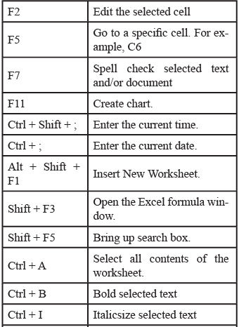
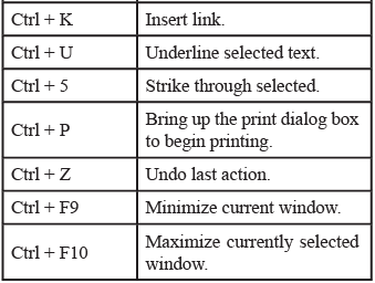
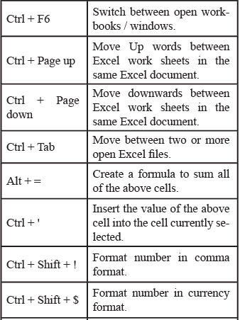
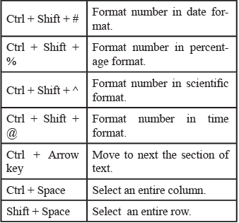
Shortcut Commands in Microsoft Excel