Random Variables | Engineering Mathematics - Civil Engineering (CE) PDF Download

Introduction

Random variable is basically a function which maps from the set of sample space to set of real numbers. The purpose is to get an idea about result of a particular situation where we are given probabilities of different outcomes. See below example for more clarity.

Example:
Suppose that two coins (unbiased) are tossed
X = number of heads. [X is a random variable or function]
Here, the sample space S = {HH, HT, TH, TT}.
The output of the function will be :
X(HH) = 2
X(HT) = 1
X(TH) = 1
X(TT) = 0

Formal Definition

X: S → R
X = random variable (It is usually denoted using capital letter)
S = set of sample space
R = set of real numbers
Suppose a random variable X takes m different values i.e. sample space X = {x1, x2, x3………xm} with probabilities P(X=xi) = pi; where 1 ≤ i ≤ m. The probabilities must satisfy the following conditions :

1. 0 <= pi <= 1; where 1 <= i <= m
2. p1 + p2 + p3 + ……. + pm = 1 Or we can say 0 ≤ pi ≤ 1 and ∑pi = 1.

Hence possible values for random variable X are 0, 1, 2.
X = {0, 1, 2} where m = 3
P(X = 0) = probability that number of heads is 0 = P(TT) = 1 / 2 * 1 / 2 = 1 / 4.
P(X = 1) = probability that number of heads is 1 = P(HT | TH) = 1 / 2 * 1 / 2 + 1 / 2 * 1 / 2 = 1 / 2.
P(X = 2) = probability that number of heads is 2 = P(HH) = 1 / 2 * 1 / 2 = 1 / 4.
Here, you can observe that

1. 0 ≤ p1, p2, p3 ≤ 1
2. p1 + p2 + p3 = 1 / 4 + 2 / 4 + 1 / 4 = 1

Example:
Suppose a dice is thrown X = outcome of the dice. Here, the sample space S = {1, 2, 3, 4, 5, 6}. The output of the function will be:

1. P(X = 1) = 1 / 6
2. P(X = 2) = 1 / 6
3. P(X = 3) = 1 / 6
4. P(X = 4) = 1 / 6
5. P(X = 5) = 1 / 6
6. P(X = 6) = 1 / 6

See if there is any random variable then there must be some distribution associated with it.

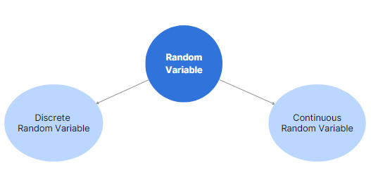
Random Variable

1. Discrete Random Variable
A random variable X is said to be discrete if it takes on finite number of values. The probability function associated with it is said to be PMF = Probability mass function.
P(xi) = Probability that X = xi = PMF of X = pi.

• 0 ≤ pi ≤ 1.
• ∑pi = 1 where sum is taken over all possible values of x.

The examples given above are discrete random variables.
Example: Let S = {0, 1, 2}Find the value of P (X = 0):
Solution: We know that sum of all probabilities is equals to 1.
==> p1 + p2 + p3 = 1
==> p1 + 0.3 + 0.5 = 1
==> p1 = 0.2

2. Continuous Random Variable
A random variable X is said to be continuous if it takes on infinite number of values. The probability function associated with it is said to be PDF = Probability density function
PDF: If X is continuous random variable.
P (x < X < x + dx) = f(x)*dx.

1. 0 ≤ f(x) ≤ 1; for all x
2. ∫ f(x) dx = 1 over all values of x

Then P (X) is said to be PDF of the distribution.

Example: Compute the value of P (1 < X < 2).
Such that f(x) = Kx³; 0 ≤ x ≤ 3 = 0; otherwise
f(x) is a density function
Solution: If a function f is said to be density function, then sum of all probabilities is equals to 1. Since it is a continuous random variable Integral value is 1 overall sample space s.
==> K  [x⁴] / 4 = 1 [Note that [x⁴] / 4 is integral of x³]
==> K  [3⁴ – 0⁴]/4 = 1
==> K = 4 / 81
The value of P (1 < X < 2) = K [X⁴] / 4 = (4 / 81) x [16 - 1] / 4 = 15 / 81.