Probability Revision Notes | Additional Topics for IIT JAM Mathematics PDF Download
Intoduction of Probability
Probability is a very popular topic of the Mathematics syllabus of the IIT JEE. It is not considered to be a very simple topic, but it is important to master the topic in order to remain competitive in IIT JEE. Majority of the students find it difficult to master this topic because their basics are not clear. In this chapter, we shall study the methodologies of computing the probability of an event, be it complex or simple. We shall try to comprehend the tools used for this purpose. In an attempt to make the subject easily comprehensible and clearly understandable a large number of illustrations and problems are selected and solved. Every aspect is fully supported by sufficient number of relevant examples. The students will note that for the understanding of the subject matter of this chapter, the knowledge of permutation and combination is essential.
We shall first throw some light on the meaning of probability and then proceed toward the various terms related to it.
Examples of Probability
- Probably, it will rain today
- It is possible that there will be drought in this area due to scanty rain
- India is likely to win the world cup
In each of the above sentences there are different degrees of certainty of results.
This degree of certainty can be measured with the help of Probability.
Hence, Probability in general terms can be described how likely something will happen.
A Simple Example of Probability
Tossing a fair (unbiased) coin. There are 2 possible outcomes
Head (H) or
Tail (T)
As the coin is unbiased, the possible outcome of ‘head’ and ‘tail’ is equally probable.
Since there are no other outcomes possible, the probability is ½ (i.e. 50%) of either “head” or “tail”.
In other words, probability that head will occur is 1 out of 2 outcomes and probability of tail is also 1 out of 2 outcomes.
Probability is a guide, it never tells us exactly or accurately what will happen, rather just an idea
For Example: When a coin is tossed 100 times, how many heads will come up?
As per our above example, probability that head turns up is ½, so expected is 50 Heads.
But when we actually try it, we might get 46 or 45 or 57 heads. But in most cases the number will be around 50.
What do you mean by the Term Probability?
In simplest possible words, probability is the degree of likeliness of the happening of an event. It is not always possible to predict an event with total certainity. In such circumstances, the concept of probability is used to predict how likely are they to happen or not. It may also be defined as a measure or estimation of likelihood of occurrence of an event. Probabilities are given a value between 0 (0% chance or will not happen) and 1 (100% chance or will happen). The higher the degree of probability, the more likely the event is to happen, or, in a longer series of samples, the greater the number of times such event is expected to happen.We disucss this in detail with the help of following examples:
1. Throwing a dice: When we throw a dice, there can be six possible outcomes. We can get any number among 1 to 6 and hence the total number of possible outcomes is 6. The probability of getting any number from 1 to 6 is therefore 1/6. But what is the probability of getting a 7 on the throw of a dice? Since it is not possible to get a 7 on a dice hence, its probability is zero.
2. Tossing a coin: When a coin is tossed, we can either get a head or tail. So, there can be two possible outcomes and the rpobability of each is ½.
Hence, P(H) = P(T) = ½.
It is clear form the above examples that probability of an event just denotes the possibility of its occurence or non-occurence. Hence, we get the following formula:
Probability of occurence of event A = P(A) = Number of favourable outcomes/ Total number of outcomes
Probability Line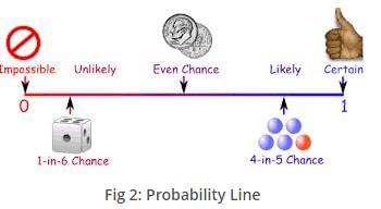
Probability is always between 0 and 1
What is Probability and Statistics?
Probability and Statistics is a branch of Mathematic s that studies the possible outcomes of events and analysis of random phenomena, interpretation and display of numerical data. The outcome of random event cannot be determined before it occurs, but it may be one of the several possible results or outcomes. The actual outcome is to be determined by chance. Probability has many applications in the field of Statistics, Science and Technology, Economics, etc.
Remark:
1. The number of outcomes favourable to A are denoted by n(A) and total number of outcomes in sample space are denoted by n(S). Hence, the above formula becomes P(A) = n(A)/n(S).
2. The probability of an event can vary between 0 to 1, i.e. 0 ≤ p ≤ 1.
3. Probability can never be negative.
4. Probability of occurence of an event = 1 – (Probability that it doesn’t occur).
Illustration 1:
A glass jar contains 5 red, 6 green, 3 blue and 8 yellow coins. If a single coin is chosen at random from the jar, what is the probability of choosing a red coin, a green coin, a blue coin or a yellow one?
Solution:
The possible outcomes of the experiment are red, green, blue and pink. Using the above mentioned formula, we have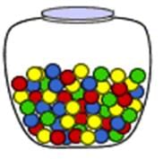
P(red) = Number of ways to chose red/ total number of coins
= 5/22
P(green) = Number of ways to chose red/ total number of coins
= 6/22
P(blue) = Number of ways to chose red/ total number of coins
= 3/22
P(yellow) = Number of ways to chose red/ total number of coins
= 8/22
This shows that the outcomes are not equally likely.
The various topics covered in this chapter are listed below:
- Experiment,Sample Space and Event
- Introduction to Probability
- Conditional Probability
- Independent events
- Bayes’ Theorem
- Binomial Distribution for successive events
- Solved Examples
All the above topics have been discussed in detail in the coming sections. Here, we shall just give a brief outline of each of them:
Experiment or Trial
An experiment or a trial refers to an action whose result is not certain. Some examples of trials include tossing a coin, throwing dice, drawing a card from a deck of cards.
Experiment: An operation which can produce some well-defined outcome(s).
There are two types of expreriment:
- Deterministic
- Random or Probabilistic
- Deterministic Experiment: The experiments which when repeated under identical conditions and produce the same result or outcome. These type of experiment have only one possible outcome and results are certain and unique
For Example: Experiments which are conducted to verify the laws of science or established laws of other areas
- An experiment conducted to verify the Newton’s law of motion.
- An experiment conducted to verify the economic law of demand
Random Experiment: If an experiment, when repeated under identical condition does not produce the same outcome every time. All the outcomes of the random experiment are known in advance, but not any specific outcome.
For Example: Throwing a die is a random experiment because we know in advance that there are only six possible outcomes of the experiment i.e. 1, 2, 3,4,5,6 but it is not possible to know which of these six numbers will finally be the result.
Thus, a random experiment is the action in which:
- All the possible results of the action are known in advance
- The exact result is unpredictable
Outcome: The result of random experiment is called as outcome of the experiment.
Sample Space
All the possible outcomes of an experiment are known as the sample space.
Example: There are 52 cards in a deck. Hence, the sample space is all 52 cards.
Sample Point
A sample space is made up of sample points which refers to just one of the possible outcome.
Eg: In a deck of cards, getting the King of Hearts is a sample point. Please note that "King" is not a sample point as there are 4 Kings which constitute 4 different sample points.
Obtaining a ‘2’ when a dice is thrown is a sample point.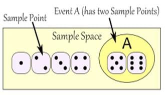
Event
A single result of an experiment is called an event. Some examples of events include getting a tail on the toss of a coin is an event.
Types of Events
Elementary Event: An outcome of a random experiment is known as an elementary event.
Example: Consider the random experiment of tossing of a coin. The possible outcomes of this experiment are head (H) or tail (T).
Thus,
E1 = Getting head (H) on the upper face of the coin,
And
E2 = Getting tail (T) on the upper face of the coin.
Then E1 and E2 are elementary events associated with the experiment
Compound Event: If an event obtained from a random experiment is by combining two or more elementary events associated to the random experiment.
Example: In a single throw of a die, the event “Getting an even number” is a compound event obtained by combining elementary events 1, 3 and 5.
Certain Event: The event which contains all the sample points of sample space is called a certain event.
Example: A random experiment of a card drawn at random from a pack of 52 cards. Let event A: card drawn is either red or black.
Therefore, Event A is a certain event
Impossible Event: An event which does not contain any sample point of the sample space S is called as impossible event. Null set Ø represents an impossible event.
Example: Let event B: die shows a number greater than 6
Therefore, B= {} = Ø
Complement of an Event
Let A be an event of Sample Space S. The set of all outcomes which are in S but not in A is called complement of the event A and is denoted by A’.
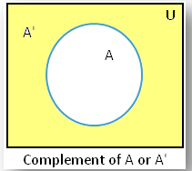 Fig 5: Complement of Event
Mutually Exclusive Events (Disjoint Events)
Let S be the sample space. A and B be two events of S. Events A and B are said to be mutually exclusive if they do not have any sample point in common.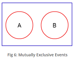
Independent Events
Two events are said to be independent of each other if the probability of the occurrence of one event does not affect the probability of the occurrence of the other event.
Example: Suppose you rolled a dice and tossed a coin. Now the probability of getting a particular number on the dice in no way influences the probability of getting a head or a tail on the coin.
Remark:
Three events A, B and C are independent if all the given conditions hold good:
P(A ∩ B) = P(A) . P(B), P(B ∩ C) = P(B) . P(C), P(C ∩ A) = P(C) . P(A)
P(A ∩ B ∩ C) = P(A).P(B).P(C)
Hence, three events are said to be independent if they are independent in pairs as well as mutually independent.
Similarly, if we have n events A1, A2, …. An, then they are said to be independent if they satisfy nC2 + nC3 + …. + nCn = 2n – n – 1 conditions.
Probability Distribution
A Probability distribution is a table or an equation that links each outcome of a statistical experiment with its probability of occurrence.
In order to understand probability distribution, it is important to understand variables, random variables and some notation
- A variable is a symbol ( A,B , x, y , etc) that can take any specified set of values
- When the value of a variable is the outcome of the statistical experiment, that variable is a random variable
X represents the random variable X
P(X) represents the probability of X
P(X=x) refers to the probability that the random variable X is equal to a particular value denoted by x
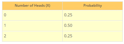
Suppose a coin is flipped 2 times. This statistical experiment can have 4 possible outcomes: HH, HT, TH, and TT. Let variable X represents the number of Heads that result from this experiment. The variable X can take the values 0, 1 or 2. In this example, X is a random variable.
A probability distribution is a table or an equation that links each outcome of a statistical experiment with its probability of occurrence. The below table shows each outcome associated with its probability with reference to the above experiment conducted with X as no of heads.
Conditional Probability
Sometimes the probability of a given event depends on the occurrence or non-occurrence of some other event.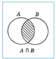
Suppose A and B are two events in a sample space S.
Let n = number of sample points in S
m1 = number of sample points in A
m2 = number of sample points in B
m12 = number of sample points in A∩B.
Then,
P(A) = m1/n, P(B) = m2/n and P(A∩B) = m12/n
The probability of A∩B, (i.e. of B) in the sample space A is m12/m1. This is the probability of B under the assumption that A takes place. It is denoted by P(B/A) and is called the conditional probability of B given that A takes place.
Therefore, P(B/A) = m12/m1 = n(A∩B)/n(A), provided n(A) ≠ 0.
Similarly, P(A/B) = m12/m2 = n(A∩B)/n(B), provided n(B) ≠ 0.
Two events A and B are said to be independent, if P(A/B)=P(A) and P(B/A) = P(B).
Bayes Theorem
In Probability, Bayes theorem describes the probability of an event, based on the prior knowledge of conditions that might be related to the event.
For Example, cancer is related to age, and then using Bayes theorem, a person’s age can be used to more accurately assess the probability that they have cancer, compared to the assessment of the probability of cancer made without knowledge of the person’s age.
The probability given under Bayes theorem is also known by the name of inverse probability, posterior probability or revised probability. This theorem finds the probability of an event by considering the given sample information; hence the name posterior probability. The Bayes theorem is based on the formula of conditional probability.
If A1, A2, A3,…..An are n mutually exclusive events from the Sample Space S, B is any other event from S and if probability of occurrence of Ai’s and probability of occurrence of B given that Ai, i=1,2,3,…n has occurred are known, then probabilities of occurrence of Ai’s given that B has occurred are given by
P(Ai/B)= P(A).P(B/Ai) ; i=1,2,3,….,n
∑ P(Ai).P(B/A)
i=1
Binomial Distribution for Successive Events
Binomial distribution is one of the most important distributions in the probability theory. The probability distribution that summarizes the likelihood that a value will take one of two independent values under a given set of parameters or assumptions is called the binomial distribution.
Let probability of success in any trial be p and that of failure be q, then
p + q = 1
Then (p + q)n = C0 Pn + C1Pn-1q +...... Crpn-rqr +...+ Cnqn
Then the probability of exactly k successes in n trials is given by
Pk = nCkqn-kpk
Assumptions of Binomial Distribution
1. The number of observations n is fixed.
2. It gives one of the two possible outcomes, say 'success' (when required event take place) and failure (when required event does not take place)
3. Each trial has the same probability of success.
4. Each trial is mutually exclusive.
5. The probability of getting at least k successes is P(x > k) = Σnx=k nCx px qn-x
6. Σnx=k nCx qn-x px = (q + p)n = 1.
7. Mean of binomial distribution is np.
8. Variance is npq,
9. Standard deviation is given by (npq)1/2, where n,p and q have their meanings as described above.
Important assumptions have been depicted below in the form of chart:
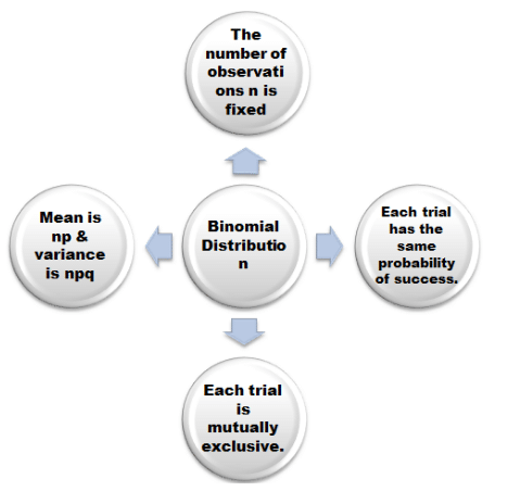
Illustration 2:
A and B are two candidates seeking admission in IIT. The probability that A is selected is 0.5 and the probability that both A and B are selected is almost 0.3. Is it possible that the probability of B getting selected is 0.9?(IIT JEE 1982)
Solution:
Let P (A) and P (B) be the probabilities of selection of A and B respectively.
P (A) = 0.5, P (A∩B) ≤ 0.3
P(A∪B) = P(A) + P(B) – P(A∩B) ≤ 1
P(B) ≤ 1 + P(A∩B) – P(A)
≤ 1 + 0.3 – 0.5 ≤ 0.8
Hence, the probability of selection of B cannot be 0.9.
Illustration 3:
A and B are two independent events. The probability that both A and B occur is 1/6 and the probability that neither of them occurs is 1/3. Find the probability of occurrence of A.
Solution:
It is given that P (A).P (B) = 1/6
And also P (Ac) P (Bc) = 1/3
This can also be written as [1-P(A)]. [1-P (B)] = 1/3
Let P(A) = x and P(B) = y
Then (1-x)(1-y) = 1/3 and xy = 1/6
Hence, 1-x-y+xy = 1/3 and xy = 1/6
x+y = 5/6 and xy = 1/6
x(5/6 – x) = 1/6
6x2 – 5x + 1 = 0.
(3x -1) (2x-1) = 0
So x = 1/3 and 1/2
Hence, the probability of A i.e. P(A) = 1/3 or ½.
Illustration 4:
In a test an examinee either guesses or copies or knows the answer to a multiple choice question with four choices. The probability that he makes a guess is 1/3 and the probability that he copies the answer is 1/6. The probability that his answer is correct given that he copied it is 1/8. Find the probability that he knew the answer to the questions given that he correctly answered it.
Solution:
let us use the following symbols for denoting the various options
G for guesses
C for copies
K denotes the possibility that the examinee knows
R if the answer is right
So, P(G) = 1/3
P(C) = 1/6
P(K) = 1- (1/3 + 1/6) =1/2
Now R = (R∩G) ∪ (R∩C) ∪ (R∩K)
P(R) = P(G) P(R/G) + P(C) P(R/C) + P(K) P(R/K) … (1)
Now, P(R/G) = 1/4
P(R/C) =1/8
P(R/K) =1
Putting this in equation (1), we obtain
P(R) = 1/3. 1/4 + 1/6.1/8 + 3/6. 1
= 1/12 +1/48 + 3/6
= 29/48
Hence, the required probability = P(K∩R)/ P(R)
= 24/29
|
2 videos|45 docs|4 tests
|
FAQs on Probability Revision Notes - Additional Topics for IIT JAM Mathematics
| 1. What is probability mathematics? |  |
| 2. How is probability calculated? |  |
| 3. What are the different types of probability? |  |
| 4. How does probability relate to statistics? |  |
| 5. What are some real-life applications of probability mathematics? |  |


