Steady-State Errors

Introduction

The deviation of the output of a control system from the desired reference in steady operation is called the steady-state error. It is commonly denoted by e_ss. Steady-state error is obtained from the error signal e(t) by using the final value theorem in the Laplace domain.

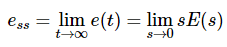
In the expression above, E(s) is the Laplace transform of the error signal e(t), and the final value theorem gives

e_ss = lim_t→∞ e(t) = lim_s→0 s E(s).

We treat steady-state errors separately for unity feedback and non-unity feedback closed-loop systems because the algebraic expressions for the error differ. The usual approach is to express E(s) in terms of R(s) and the open-loop transfer function and then apply the final value theorem.

Steady-State Errors for Unity Feedback Systems

Consider a closed-loop control system with unity negative feedback as shown below.

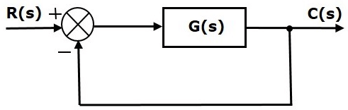
Let the Laplace transforms of the reference input and the output be R(s) and C(s) respectively.

• R(s) - Laplace transform of reference input r(t).
• C(s) - Laplace transform of output c(t).

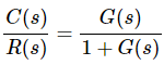
The closed-loop transfer function for a system with forward path G(s) and unity negative feedback is

The error at the summing point is

E(s) = R(s) - C(s)

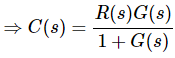
Substitute the expression for C(s) from the closed-loop transfer function into the expression for E(s).

C(s) = G(s) R(s) / [1 + G(s)]

E(s) = R(s) - G(s) R(s) / [1 + G(s)]

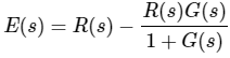
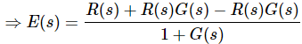
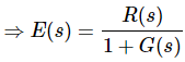
Factor R(s) to obtain E(s) in a convenient form for the final value theorem.

E(s) = R(s) / [1 + G(s)]

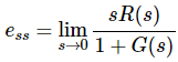
Apply the final value theorem to obtain steady-state error for a given reference R(s).

For standard reference inputs, steady-state errors are commonly expressed using error constants. The standard relationships are usually summarised in a table that lists the steady-state error for a unit step, unit ramp and unit parabolic input in terms of the open-loop error constants.

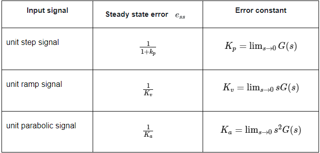
Here the error constants are defined as follows.

• Position error constant K_p = lim_s→0 G(s).
• Velocity error constant K_v = lim_s→0 s·G(s).
• Acceleration error constant K_a = lim_s→0 s²·G(s).

Using these constants, the steady-state error for standard inputs is given by the table shown above. For clarity:

• For a unit step input R(s) = 1/s, e_ss = 1 / (1 + K_p).
• For a unit ramp input R(s) = 1/s², e_ss = 1 / K_v, if K_v is finite.
• For a unit parabolic input R(s) = 1/s³, e_ss = 1 / K_a, if K_a is finite.

Note

• If any of the standard input signals has amplitude other than unity, multiply the corresponding steady-state error by that amplitude.
• Steady-state error is not defined for a unit impulse input in the usual sense because the impulse exists only at t = 0 and the final value (t → ∞) comparison is not meaningful.

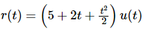
Example

Find the steady-state error for a unity negative feedback system when the input signal is a combination of step, ramp and parabolic components as shown below.

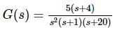
Let the forward path transfer function of the system be as shown.

Compute error constants for the system and the steady-state error contributed by each component of the input. The standard tabulation of error constants and the resulting steady-state errors for the three components is shown below.

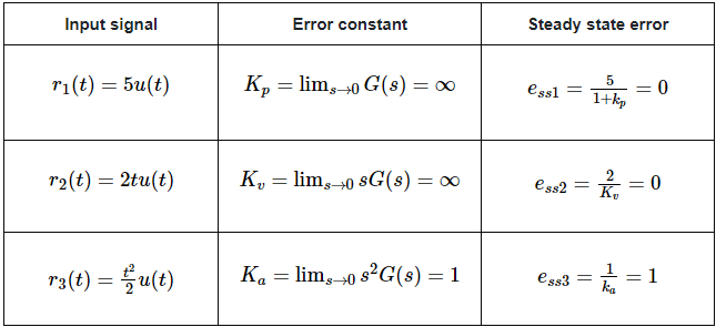
The overall steady-state error is the algebraic sum of the steady-state errors due to the individual components of the input.

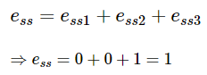
Therefore, for this example, the steady-state error e_ss is 1.

Steady-State Errors for Non-Unity Feedback Systems

Consider a closed-loop control system with a non-unity feedback H(s) as shown below.

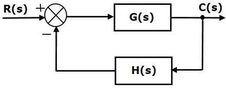
It is most convenient to compute steady-state error using the standard unity-feedback relationships. To do that, we convert the non-unity feedback structure into an equivalent unity feedback form by manipulating the block diagram.

One common method is to move H(s) into the forward path by algebraic block reduction and to introduce an equivalent single forward-path block so that the feedback becomes unity. The conversion process is illustrated in the following figures.

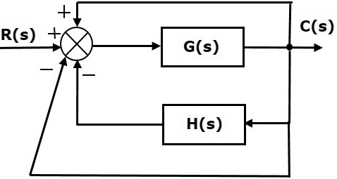
Simplify the block diagram by keeping a unity negative feedback loop and combining the remaining forward-path elements into a single equivalent transfer function. The simplified equivalent block diagram is:

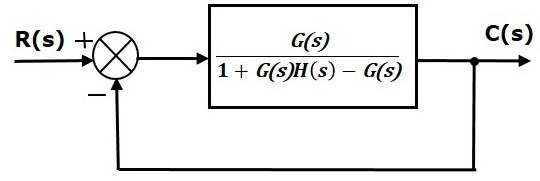
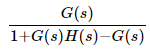
In this equivalent unity-feedback diagram the single forward block has the transfer function shown below (replace this block where the original forward path and feedback have been combined). Use this transformed forward transfer function in place of G(s) for steady-state error calculations.

After the transformation, calculate error constants and steady-state errors exactly as done for unity feedback systems, using the equivalent forward transfer function.

Note: It is meaningless to compute steady-state error for an unstable closed-loop system. Therefore check the closed-loop stability first and compute steady-state errors only for stable closed-loop systems. Stability analysis is treated in the next chapter.

Practical remarks and applications

• System type and steady-state performance: The number of pure integrators in the open-loop forward path (that is, the system type) largely determines which inputs can be tracked with zero steady-state error. A type 0 system cannot track a ramp with zero error, a type 1 system can track a step with zero error, and a type 2 system can track a ramp with zero error, etc.
• Controller design: Adding integral action in a controller increases system type and reduces steady-state error for certain reference inputs, but it may affect stability and transient response. Design always balances steady-state requirements and dynamic behaviour.
• Use of error constants: Error constants K_p, K_v, K_a provide quick measures of steady-state performance without computing full time-domain responses; they are widely used in preliminary design and analysis.
• Verification: After analytic computation of e_ss, verify results by simulation or by time-domain analysis to ensure the closed-loop system is stable and assumptions (such as low-frequency approximations) are valid.

Summary

Steady-state error quantifies the long-time difference between reference and output. For unity feedback systems, derive E(s) = R(s) / [1 + G(s)] and use e_ss = lim_s→0 sE(s). Use error constants K_p, K_v, K_a to obtain closed-form steady-state errors for standard inputs. For non-unity feedback systems, convert to an equivalent unity-feedback form before applying the same formulae. Always confirm closed-loop stability before interpreting steady-state errors.