Symmetrical Bending - Civil Engineering (CE) PDF Download

Symmetrical Bending
Here we assume that the beam is loaded along a single symmetric plane of the cross section. Without loss of generality we assume that this symmetric loading plane is the xy plane of the beam. For illustration, let us assume that the cross section of the beam is rectangular with depth 2c and width 2b and length 2l as shown in figure 8.2. Further, let us assume that the beam is simply supported at the ends A and B and is subjected to a uniform pressure loading W on its top surface as pictorially represented in figure 8.2. We derive the strength of materials solution before obtaining the 2 dimensional elasticity solution for this problem. While the strength of materials solution is generic, in that it is applicable for any cross section, elasticity solution is specific for rectangular cross section alone.
Strength of materials solution
Here the displacement approach is used to obtain the solution. Hence, the main assumption here is regarding the displacement field. The assumption
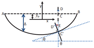
Figure 8.3: Schematic of deformation of a beam. ACB beam before deformation, AC0B beam after deformation.
is that sections that are plane and perpendicular to the neutral axis (to be defined shortly) of the beam remain plane and perpendicular to the deformed neutral axis of the beam, as shown in figure 8.3. Hence, the displacement field is,
where ∆(x) is a function of x denotes the displacement of the neutral axis of the beam along the ey direction and yo is a constant. yo is the y coordinate of the neutral axis before the deformation in the chosen coordinate system and is a constant because the beam is straight. Before proceeding further let us see why the x component of the displacement is as given. The line D'E in figure 8.3 denotes the magnitude of the x component of the displacement. D'E = C'D' sin(θ) which is approximately computed as D'E = CDθ, assuming small rotations and that there is no shortening of line segments along the ey direction so that C'D' = CD. Now if y coordinate of C is yo and that of D is y, then the length of line segment CD = (y − yo). Similarly, from the assumption that the plane sections perpendicular to the neutral axis remain perpendicular to the deformed neutral axis, θ =  , the slope of the tangent of the deformed neutral axis, as shown in the figure 8.3. Therefore D'E = (y − yo) and the x component of the displacement is −D'E since, it is in a direction opposite to the ex direction.
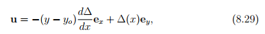
Now, the gradient of the displacement field for the assumed displacement (8.29) is
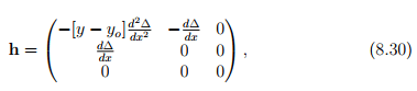
and therefore the linearized strain is
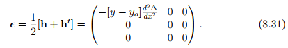
Using the one dimensional constitutive relation, σ(n) = E€(n) , where σ(n) and E€(n) are the normal stress and strain along the direction n, we obtain
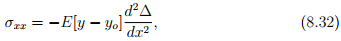
where we have equated the normal stress and strain along the ex direction. Substituting equation (8.32) in the equation (8.3) we obtain
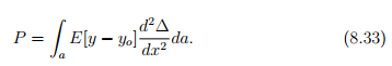
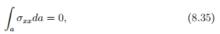
Since, in a beam there would be no net applied axial load P = 0. Solving equation (8.33) for yo under the assumption that no net axial load is applied,
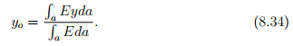
If the beam is also homogeneous then Young’s modulus, E is a constant and therefore, 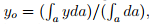 centroid of the cross section. Since, we have assumed that there is no net applied axial load, i.e.,
equation (8.9) can be written as,
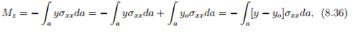
where yo is a constant given in equation (8.34). Substituting equation (8.32) in equation (8.36) we obtain,
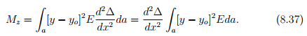
If the cross section of the beam is homogeneous, the above equation can be written as,
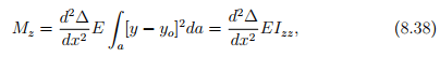
where,
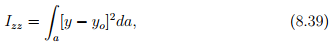
is the moment of inertia about the z axis.
Combining equations (8.37) and (8.32) we obtain for inhomogeneous beams
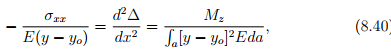
where yo is as given in equation (8.34). Combining equations (8.38) and (8.32) we obtain for homogeneous beams
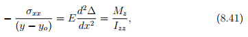
where yo is the y coordinate of the centroid of the cross section which can be taken as 0 without loss of generality provided the origin of the coordinate system used is located at the centroid of the cross section.
Next, we would like to define neutral axis. Neutral axis is defined as the line of intersection of the plane on which the bending stress is zero (y = yo) and the plane along which the resultant load acts.
Equations (8.40) and (8.41) relate the bending stresses and displacement to the bending moment in an inhomogeneous and homogeneous beam respectively and is called as the bending equation. While these equations are sufficient to find all the stresses in a beam subjected to a constant bending moment, one further needs to relate the shear stresses to the shear force that arises when the beam is subjected to a bending moment that varies along the longitudinal axis of the beam. This we shall do next.
Consider a section of the beam, pqrs as shown in figure 8.4 when the beam is subjected to a bending moment that varies along the longitudinal
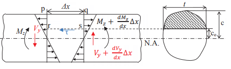
Figure 8.4: Schematic of stresses acting on a beam subjected to varying bending moment
axis of the beam. For the force equilibrium of section pqrs, the shear stress, τ , as indicated in the figure 8.4 should be
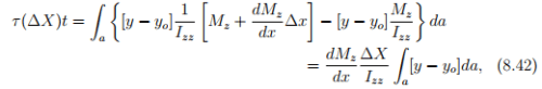
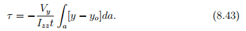
where the integration is over the cross sectional area above the section of interest, i.e., the shaded area shown in figure 8.4 and t is the width of the cross section at the section of interest. Substituting equation (8.18) in (8.42) and simplifying we obtain,
Having obtained the magnitude of this shear stress, next we discuss the direction along which this acts. For thick walled sections with say, l/b < 20, as in the case of well proportioned rectangular beams, this shear stress is the σxy (and the complimentary σyx) component. For thin walled sections, this shear stress would act tangential to the profile of the cross section as shown in the figure 8.5b and figure 8.5c. Thus it has both the σxy and σxz shear components acting on these sections.
2D Elasticity solution
While the strength of material solution is generic in that it can be used for While the strength of material solution is generic in that it can be used for
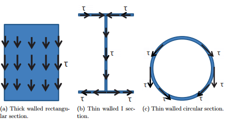
Figure 8.5: Direction of the shear stresses acting on a cross section of a beam subjected to varying bending moment
its plane of symmetry, 2D elasticity solution has to be developed for specific cross sections and loading scenarios. Consequently, we assume that the cross section is rectangular in shape with width 2b and depth 2c. Thus, the body is assumed to occupy the region in the Euclidean point space defined by B = {(x, y, z)| − l ≤ x ≤ l, −c ≤ y ≤ c, −b ≤ z ≤ b} before the application of the load. Using the stress formulation introduced in chapter 7, we study the response of this body subjected to three types of load.
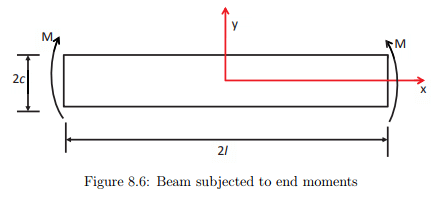
Pure bending of a simply supported beam Consider the case of a straight beam subject to end moments as shown in figure 8.6. It can be seen from the figure that the top and bottom surfaces are free of traction, i.e.
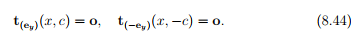
The surfaces defined by x = ±l has traction on its face such that the net force is zero but it results in a bending moment, Mz. Representing these
conditions mathematically,
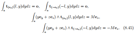
Thus, the exact point wise loading on the ends is not considered and only the statically equivalent effect is modeled. Consequently, the boundary conditions on the ends of the beam have been relaxed, and only the statically equivalent condition will be satisfied. This fact leads to a solution that is not necessarily valid at the ends of the beam and could result in more than one stress field satisfying the prescribed conditions.
Assuming the state of stress to be plane, such that
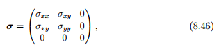
the boundary condition (8.44) translates into requiring,
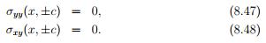
For the assumed state of stress (8.46) the boundary condition (8.45) requires,
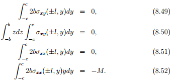
Recognize that condition (8.50) holds irrespective of what the variation of the shear stress σxy is.
As discussed in detail in chapter 7 (section 7.3.2), for stress formulation, we assume that the Cartesian components of stress are obtained from a potential, φ = φˆ(x, y), called the Airy’s stress function through
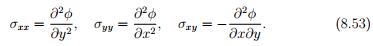
Then, we have to find the potential such that it satisfies the boundary conditions (8.47) through (8.52) and the bi-harmonic equation, ∆(∆(φ)) = 0. We express φ as a power series:
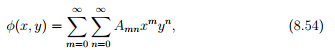
where Amn are constant coefficients to be determined from the boundary conditions and the requirement that it satisfy the bi-harmonic equation. The choice of the stress function is based on the fact that a third order Airy’s stress function will give rise to a linear stress field, and this linear boundary loading on the ends x = ±l, will satisfy the requirements (8.49) through (8.52). Based on this observation, we choose the Airy’s stress function as

Then, the stress field takes the form

Substituting the above stress in boundary conditions (8.47) and (8.48) we find that A30 = A21 = A12 = 0. Thus, the Airy’s stress function reduces to,
φ = A03y3 , (8.57)
and the stress field becomes
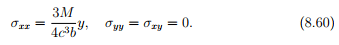
σxx = 6A03y, σyy = σxy = 0. (8.58)
Substituting (8.60) in the boundary conditions (8.49) through (8.52), we find that (8.49) through (8.51) are satisfied identically and (8.52) requires,
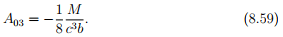
It can be verified that the Airy’s stress function (8.57) satisfies the biharmonic equation trivially. Substituting (8.59) in (8.58) we obtain,
Using the 2 dimensional Hooke’s law (7.49), the strain field corresponding to the stress field (8.60) is computed to be
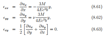
Integrating (8.61) we obtain
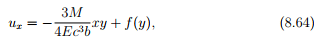
where f is an arbitrary function of y. Similarly, integrating (8.62) we obtain
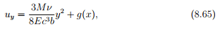
where g is an arbitrary function of x. Substituting equations (8.64) and (8.65) in equation (8.63) and simplifying we obtain
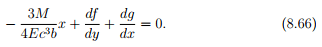
For equation (8.66) to hold,
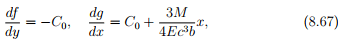
where C0 is a constant. Integrating (8.67) we obtain

where C1 and C2 are integration constants. Substituting (8.68) in equations (8.64) and (8.65) we obtain

The constants Ci ’s are to be evaluated from displacement boundary conditions. Assuming the beam to be simply supported at the ends A and B, we require
uy(±l, 0) = 0, and ux(−l, 0) = 0, (8.70)
where we have assumed the left side support to be hinged (i.e., both the vertical and horizontal displacement is not possible) and the right side support to be a roller (i.e. only vertical displacement is restrained). Substituting (8.69) in (8.70) we obtain
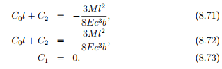
Solving the equations (8.71) and (8.72) for C0 and C2 we obtain
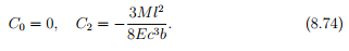
Substituting, equations (8.73) and (8.74) in the equation (8.69) we obtain the displacement field as,

If the displacement boundary condition is different, then the requirement (8.70) will change and hence the displacement field. We now wish to compare this elasticity solution with that obtained by strength of materials approach. The bending equation (8.41), for rectangular cross section being studied and the constant moment case reduces to
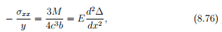
where we have used the fact that for a rectangular cross section of depth 2c and width 2b, Izz = 4c3 b/3 and that yo = 0 as the origin is at the centroid of the cross section. Using the first equality in equation (8.76) we obtain the stress field as,
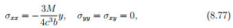
Comparing equations (8.60) and (8.77) we find that the stress field is the same in both the approaches. Then, using the last equality in equation (8.76) we obtain,
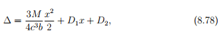
where D1 and D2 are integration constants to be found from the displacement boundary condition (8.70). This simply supported boundary condition requires that ∆(±l) = 0, i.e.,
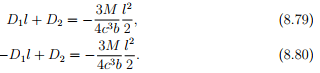
Solving the above equations we obtain,
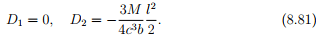
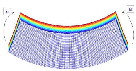
Figure 8.7: Deformed shape of a beam subjected to pure bending as obtained from the elasticity solution
Substituting (8.81) in (8.78) and the resulting equation in (8.29) we obtain
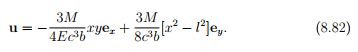
Comparing the strength of materials displacement field (8.82) with that of the elasticity solution (8.75) we find that the x component of the displacement field is the same in both the cases. However, while the y component of the displacement is in agreement with the displacement of the neutral axis, i.e., when y = 0, it is not in other cases. This is understandable, as in the strength of material solution we ignored the Poisson’s effect and used only a 1D constitutive relation. This means that the length of the filaments oriented along the y direction changes in the elasticity solution, which is explicitly assumed to be zero in the strength of materials solution. Figure 8.7 plots the deformed shape of a beam subjected to pure bending as obtained from the elasticity solution.
We shall find that this near agreement of the elasticity and strength of materials solution for pure bending of the beam does not hold for other loadings, as we shall see next.
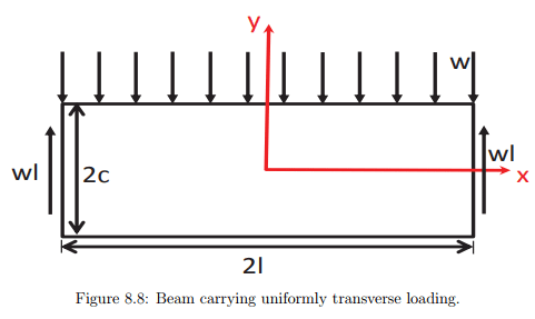
Simply supported beam subjected to uniformly distributed transverse loading
The next problem that we solve is that of a beam carrying a uniformly distributed transverse loading ω along its top surface,as shown in Figure 8.8. As before the traction boundary conditions for this problem are
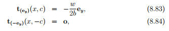
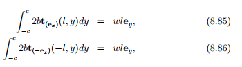
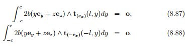
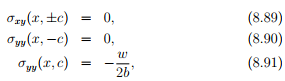
While exact point wise conditions are specified on the top and bottom surfaces, at the right and left surfaces the resultant horizontal axial force and moment are set to zero and the resultant vertical shear force is specified such that it satisfies the overall equilibrium. As before assuming plane stress conditions, (8.46), the boundary conditions (8.83) through (8.88) evaluates to,
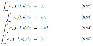
Thus, we have to chose Airy’s stress function such that conditions (8.89) through (8.95) holds along with the bi-harmonic equation. Seeking Airy’s stress function in the form of the polynomial (8.54), we try the following form,
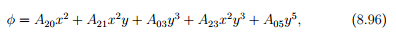
where Aij ’s are constants. For this polynomial to satisfy the bi-harmonic equation,
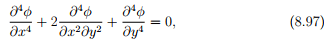
it is required that
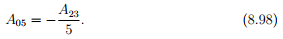
For this assumed form for the Airy’s stress function (8.96), the stress field found using equation 8.53 is,
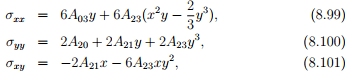
where we have used (8.98).
Substituting equation (8.101) in the boundary condition (8.89) we obtain,

Then, using equation (8.100) in the boundary conditions (8.90),(8.91) we obtain,
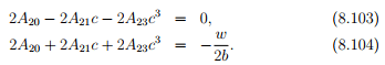
Solving the above three equations for the constants A20, A21 and A23, we obtain
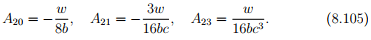
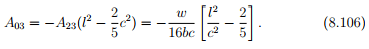
Next, substituting equation (8.99) in the boundary condition (8.92) we find that it holds for any choice of the remaining constant, A03. Similarly, when the constants, Aij are as given in (8.105), the shear stress (8.101) satisfies the boundary conditions (8.93) and (8.94). Thus, substituting equation (8.99) in the boundary condition (8.95) we obtain
Thus, the assumed form for the Airy’s stress function (8.96) with the appropriate choice for the constants, satisfies the required boundary conditions and the bi-harmonic equation and therefore is a solution to the given boundary value problem.
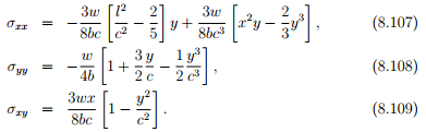
Substituting the values for the constants from equations (8.105) and (8.106) in equations (8.99) through (8.101), the resulting stress field can be written as
Having computed the stress fields, next we determine the displacement field. As usual, we use the 2 dimensional constitutive relation (7.49) to obtain the strain field as
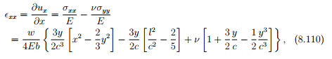
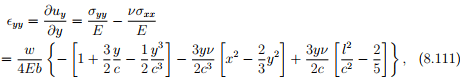
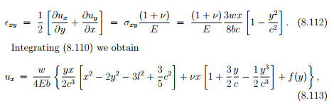
where f(y) is a yet to be determined function of y. Similarly integrating (8.111),
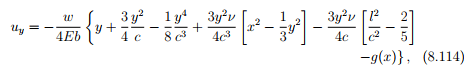
where g(x) is a yet to be determined function of x. Substituting equations (8.113) and (8.114) in (8.112) and simplifying we obtain
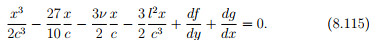
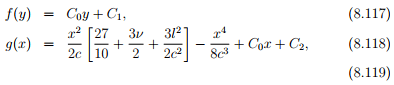
For equation (8.115) to hold,

where C0 is a constant. Integrating the differential equation (8.115) we obtain
where C1 and C2 are constants to be determined from the displacement boundary condition. Assuming the beam to be simply supported at the ends A and B, we require
uy(±l, 0) = 0, and ux(−l, 0) = 0, (8.120)
where we have assumed the left side support to be hinged (i.e., both the vertical and horizontal displacement is not possible) and the right side support to be a roller (i.e. only vertical displacement is restrained). Substituting (8.114) and (8.118) in (8.120a) we obtain
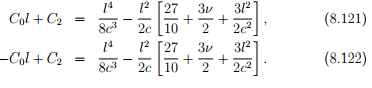
Solving equations (8.121) and (8.122) for C0 and C2,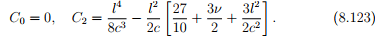
Substituting equations (8.113), (8.117) and (8.123) in (8.120b), we obtain
C1 = −νl. (8.124)
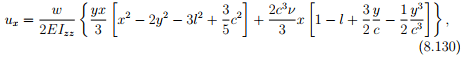
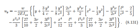
Thus, the final form of the displacements is given by
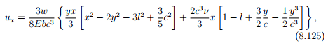
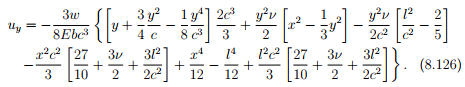
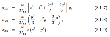
In order to facilitate the comparison of this elasticity solution with that obtained from the strength of materials approach, we rewrite the stress and displacements field obtained using the elasticity approach in terms of the moment of inertia of the rectangular cross section of depth 2c and width 2b, Izz = 4bc3/3, as
Now, we obtain the stress and displacement field from the strength of materials approach. The bending equation (8.41) for this boundary value problem reduces to
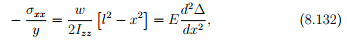
where we have taken yo = 0 as the origin of the coordinate system coincides with the centroid of the cross section and substituted for bending moment,
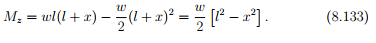
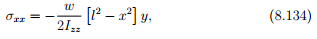
From the first equality in equation (8.132) we obtain,
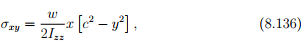
Using the equation (8.43) the shear stress, σxy for this cross section and loading is estimated as,
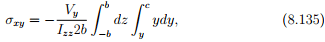
where we have used yo = 0. Noting that Vy = wl−w(l+x) = −wx, equation (8.135) simplifies to
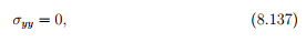
In strength of materials solution we do not account for the variation of the σyy component of the stress. Hence,
From solving the ordinary differential equation in the last equality in equation (8.132) we obtain,
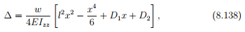
where D1 and D2 are constants to be found from the displacement boundary condition (8.120). The boundary condition (8.120a) requires that
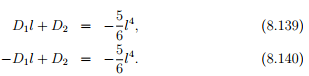
Solving equations (8.139) and (8.140) for the constants D1 and D2 we obtain
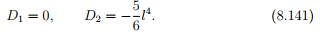
Substituting (8.141) in equation (8.138) we obtain
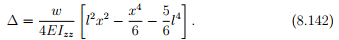
Hence the displacement field in a simply supported beam subjected to transverse loading obtained from strength of materials approach is,

Before concluding this section let us compare the 2 dimensional elasticity solution with the strength of material solution. Comparing equations (8.136) with equation (8.129), we find that identical shear stress, σxy variation is obtained in both the approaches. However, comparing equations (8.134) and (8.127) we find that the expression for the bending stress, σxx obtained by both these approaches are different. First observe that in strength of materials solution σxx(±l, y) = 0. However, in the elasticity solution, σxx(±l, y) = wy[c 2/5 − y 2/3]/Izz. Figure 8.9 plots the variation of σxx(±l, y)2b/w with respect to y/c. Moreover, at any section we find that the bending stress, σxx varies nonlinearly with respect to y in the elasticity solution. To understand how different the elasticity solution is from the strength of materials solution, in figure 8.10 we plot both the variation of the bending normal stress, σxx(0, y)2b/w as a function of y/c for various values of l/c. It can be seen from the figure that for values of l/c ≤ 1 the differences are significant but as the value of l/c tends to get larger the differences diminishes. Also notice that the maximum bending stress max(σxx(0, y)) varies quadratically as a function of l/c. In figure 8.11 we plot the variation of the stress σyy2b/w with y/c to find that its magnitude is less than 1. Thus, for typical beams with l/c > 10, the bending stresses σxx is 100 times more than these other stresses that they can be ignored, as done in strength of materials solution. Having examined the difference in the stresses let us now examine the displacements. The maximum deflection of the neutral axis of the beam in the elasticity solution is

obtained from equation (8.131). The corresponding value calculated from strength of materials solution (8.142) is
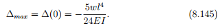
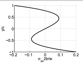
Figure 8.9: Variation of the stress σxx at the supports along the depth of the simply supported beam subjected to transverse loading
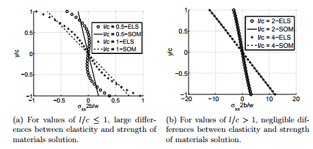
Figure 8.10: Variation of the stress σxx at mid span of a simply supported beam subjected to transverse loading

Figure 8.11: Variation of the stress σyy along the depth of the simply supported beam subjected to transverse loading
Comparing equations (8.144) and (8.145) it can be seen that when l/c 1 the results are approximately the same. Thus, again we find that for long beams with l/c > 10 the strength of materials solution is close to the elasticity solution. Note that from equation 8.125, the x component of displacement indicates that plane sections do not remain plane. However, for well proportioned beams, i.e. beams with l/c > 10, the deviation from being plane is insignificant.
Simply supported beam subjected to sinusoidal loading
Finally, we consider a simply supported rectangular cross section beam subjected to sinusoidally varying transverse load along its top edge as shown in Fig 8.12. Now, we shift the coordinate origin to the left end surface of the beam. Consequently, the beam in its initial state is assumed to occupy a region in the Euclidean point space defined by
B = {(x, y, z)|0 ≤ x ≤ 2l, −c ≤ y ≤ c, −b ≤ z ≤ b}.
The traction boundary conditions for this problem are
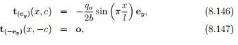
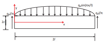
Figure 8.12: Simply supported beam subjected to sinusoidally varying transverse load
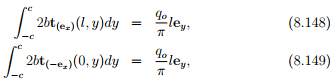
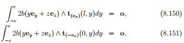
The conditions (8.146) through (8.151) on assuming that the beam is subjected to a plane state of stress, translates into requiring
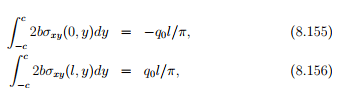
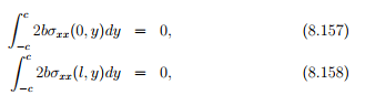
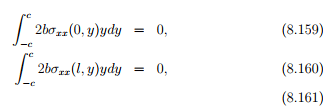
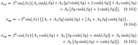
As before, we solve this boundary value problem using stress approach. Towards this, we assume the following form for the Airy’s stress function

where Ai ’s are constants to be determined from boundary conditions. It is straightforward to verify that the above choice of Airy’s stress function, (8.162) satisfies the bi-harmonic equation. Then, the Cartesian components of the stress for the assumed Airy’s stress function (8.162) is
Now applying the boundary condition we evaluate the constants, Ai ’s. The condition 8.152 implies that
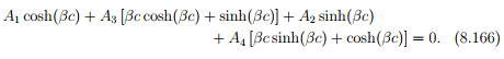
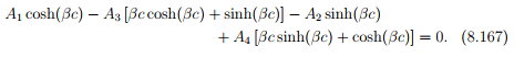
Adding equations (8.166) and (8.167) we obtain,

Subtracting equations (8.166) and (8.167) we obtain,

We write A1 in terms of A4 using equation (8.168) as

Similarly, we write A2 in terms of A3 using equation (8.169) as

Substituting equations (8.170) and (8.171) in (8.164)
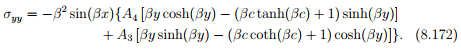
Applying boundary condition (8.154) we obtain a relation between A3 and A4 as

The boundary condition (8.153) requires
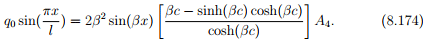
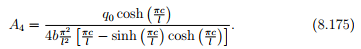
In order for equation 8.174 to be true for all x, β = π/l, and so A4 is determined as,
It can be verified that for these choice of constants, boundary conditions It can be verified that for these choice of constants, boundary conditions that satisfies the bi-harmonic equation and the traction boundary conditions and therefore is a solution to the boundary value problem. The displacements are determined through integration of the strain displacement relations. Since the steps in its computation is same as in the above two examples, only the final results are recorded here
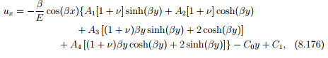
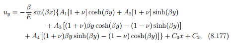
where Ci ’s are constants to be determined from displacement boundary conditions. As before, to model a simply supported beam, we choose displacement boundary conditions as
ux(0, 0) = uy(0, 0) = uy(l, 0) = 0. (8.178)
The constant Ci ’s determined using the above displacement conditions is
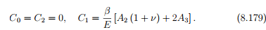
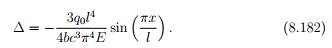
For the case when l >> c, we approximately compute A4 as A4 ≈ −3q0l5/8bc3π5 , and so the equation (8.180) becomes

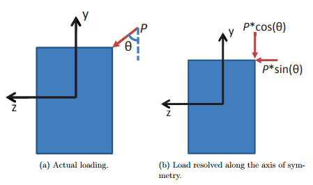
Figure 8.13: Schematic of transverse loading of a beam with rectangular cross section Without going into the details, the vertical deflection of the beam computed using strength of materials approach is,
When l/c > 10 it can be seen that both the elasticity and strength of materials solution is in agreement as expected.
FAQs on Symmetrical Bending - Civil Engineering (CE)
| 1. What is symmetrical bending? |  |
| 2. What are the properties of a structure experiencing symmetrical bending? | |
| 3. How does symmetrical bending affect the structural integrity of an object? | |
| 4. What are some common applications of symmetrical bending in engineering and construction? | |
| 5. How can the concept of symmetrical bending be applied to real-life scenarios? | |


video lectures
,MCQs
,Important questions
,Objective type Questions
,Symmetrical Bending - Civil Engineering (CE)
,Symmetrical Bending - Civil Engineering (CE)
,shortcuts and tricks
,Summary
,ppt
,Free
,Extra Questions
,study material
,Viva Questions
,mock tests for examination
,Semester Notes
,Previous Year Questions with Solutions
,Exam
,Sample Paper
,practice quizzes
,past year papers
,Symmetrical Bending - Civil Engineering (CE)
;


Symmetrical Bending Free PDF Download
Importance of Symmetrical Bending
Symmetrical Bending Notes
Symmetrical Bending Civil Engineering (CE) Questions
Study Symmetrical Bending on the App
|
© EduRev
|
Education Revolution
|


|


within 7 days!