Taylor’s Square Root of Time Fitting Method - Determination of Coefficient of Consolidation of Soil, | Soil Mechanics Notes- Agricultural Engineering PDF Download
Taylor’s Square Root of Time Fitting Method
From the oedometer test (explained in Lesson 23) the dial reading (settlement) corresponding to a particular time is measured. From the measured data, dial reading vs \[\sqrt {Time}\] graph can be drawn (as shown in Figure 24.1). A straight line can be drawn passing through the points on initial straight portion of the curve (as shown in Figure 24.1). The intersection point between the straight line and the dial reading axis is denoted as R0 which is corrected zero reading i.e U = 0%. Starting from R0, draw another straight line such that its abscissa is 1.15 times the abscissa of first straight line. The intersection point between the second straight line and experimental curve represents theR90 and corresponding \[\sqrt {{t_{90}}}\] is determined. Thus, the time required (t90) for 90% consolidation is calculated. The Coefficient of consolidation (cv) is determined as:
\[{c_v}={{{T_v}{H^2}} \over t}\] (24.1)
where H is the thickness of the soil sample, t is required time. Tv is the vertical time factor and can be determine as:
\[{T_v}=\left({{\pi\over 4}}\right){U^2}\quad \quad if\;U \le 60\% \] % (24.2)
\[{T_v}=1.781 - 0.933{\log _{10}}(100 - U)\quad \quad if\;U > 60\% \] % (24.3)
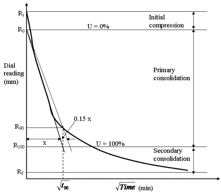
Fig. 24.1. Taylor’s Square Root of Time Fitting Method.
FAQs on Taylor’s Square Root of Time Fitting Method - Determination of Coefficient of Consolidation of Soil, - Soil Mechanics Notes- Agricultural Engineering
| 1. What is Taylor's Square Root of Time fitting method? |  |
| 2. How is the coefficient of consolidation of soil determined using Taylor's Square Root of Time fitting method? | |
| 3. Why is Taylor's Square Root of Time fitting method used to determine the coefficient of consolidation? | |
| 4. What are the advantages of using Taylor's Square Root of Time fitting method for determining the coefficient of consolidation? | |
| 5. What are some limitations of Taylor's Square Root of Time fitting method in determining the coefficient of consolidation? | |

|
5.4K Views |

|
4.68/5 Rating |

|
Dec 23, 2024 Last updated |

|
Explore Courses for Agricultural Engineering exam
|
|
practice quizzes
,Objective type Questions
,Exam
,Sample Paper
,mock tests for examination
,Extra Questions
,ppt
,| Soil Mechanics Notes- Agricultural Engineering
,Taylor’s Square Root of Time Fitting Method - Determination of Coefficient of Consolidation of Soil
,Taylor’s Square Root of Time Fitting Method - Determination of Coefficient of Consolidation of Soil
,past year papers
,video lectures
,Taylor’s Square Root of Time Fitting Method - Determination of Coefficient of Consolidation of Soil
,shortcuts and tricks
,| Soil Mechanics Notes- Agricultural Engineering
,Viva Questions
,MCQs
,| Soil Mechanics Notes- Agricultural Engineering
,Summary
,study material
,Important questions
,Free
,Previous Year Questions with Solutions
,Semester Notes
;


Taylor’s Square Root of Time Fitting Method - Determination of Coefficient of Consolidation of Soil, Free PDF Download
Importance of Taylor’s Square Root of Time Fitting Method - Determination of Coefficient of Consolidation of Soil,
Taylor’s Square Root of Time Fitting Method - Determination of Coefficient of Consolidation of Soil, Notes
Taylor’s Square Root of Time Fitting Method - Determination of Coefficient of Consolidation of Soil, Agricultural Engineering Questions
Study Taylor’s Square Root of Time Fitting Method - Determination of Coefficient of Consolidation of Soil, on the App
|
© EduRev
|
Education Revolution
|


|


