Techniques to Solve Boundary Value Problems - Civil Engineering (CE) PDF Download

Techniques to solve boundary value problems
Depending on the boundary condition specified the solution can be found using one of the following two techniques. Outline of these methods is presented next.
Displacement method
Here we take the displacement field as the basic unknown that need to be determined. Then using this displacement field we find the strain using the strain displacement relation (7.1). The so computed strain is substituted in the constitutive relation written using Lam`e constants (7.2) to obtain
σ = λdiv(u)1 + µ [grad(u) + grad(u)t ], (7.14)
where we have used the definition of divergence operator, (2.208) and the property of the trace operator (2.67). Substituting (7.14) in the reduced property of the trace operator (2.67). Substituting (7.14) in the reduced and the body is in static equilibrium, (7.5) we obtain

where we have used equation (3.31) to write the acceleration in terms of the displacement and  denotes the total time derivative. In addition, to obtain the equation (7.15), we have used the following identities:
1. Since divergence is a linear operator

2. It follows from equation (2.218) that
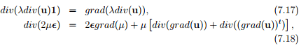
where we have used the fact that div is a linear operator and 1m = m when m is any vector and 1 is the second order identity tensor.
3. From the identity (2.222) it follows that,

4. Using definition of the Laplace operator (2.212)
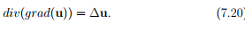
5. Using the identity (2.211) we note that

Thus, we obtain (7.15) by substituting successive substitution of equations (7.17) through (7.21) in (7.16).
In order to simplify equation (7.15), we make the following assumptions:
1. The body is homogeneous.Hence λ and μ are constants
2. Body forces can be ignored
3. Body is in static equilibrium under the applied traction In lieu of these assumptions, equation (7.15) reduces to
In lieu of these assumptions, equation (7.15) reduces to
(λ + µ)grad(div(u)) + µ∆u = o. (7.22)
If body forces cannot be ignored but the other two assumptions hold, then (7.15) reduces to
(λ + µ)grad(div(u)) + µ∆u + ρb = o. (7.23)
In this course, we attempt to find the displacement field that satisfies (7.22) along with the prescribed boundary conditions. We compute the stress field corresponding to the determined displacement field, using equation (7.2) where the strain is related to the displacement field through equation (7.1). We illustrate this method in section 7.4.1.
Stress method
Here we use stress as the basic unknown that needs to be determined. This method is applicable only for cases when the inertial forces (ρa) can be neglected. Since, we have assumed stress as the basic unknown, we want to express the compatibility conditions (7.7) through (7.12) in terms of the stresses. For this we compute the strains in terms of the stresses using the constitutive relation (7.4) and substitute in the compatibility conditions to obtain the following 6 equations:
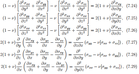
where we have assumed that the body is homogeneous and hence Young’s modulus, E and Poisson’s ratio, ν do not vary spatially. Now, we have to find the 6 components of the stress such that the 6 equations (7.24) through (7.29) holds along with the three equilibrium equations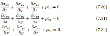
where bi ’s are the Cartesian components of the body forces. The above equilibrium equations (7.30) through (7.32) are obtained from (7.5) by setting a = o.
If the body forces could be obtained from a potential, 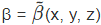 called as the load potential, as
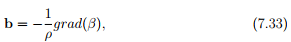
then the Cartesian components of the Cauchy stress could be obtained from a potential, φ = φ˜(x, y, z) called as the Airy’s stress potential and the load potential, β as,
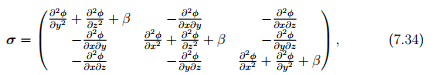
so that the equilibrium equations (7.30) through (7.32) is satisfied for any choice of φ. Substituting for the Cartesian components of the stress from equation (7.34) in the compatibility equations (7.24) through (7.29) and simplifying we obtain:
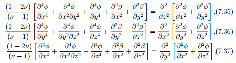
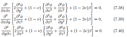
Thus, a potential that satisfies equations (7.35) through (7.40) and the prescribed boundary conditions is said to be the solution to the given boundary value problem. Once the Airy’s stress potential is obtained, the stress field could be computed using (7.34). Using this stress field the strain field is computed using the constitutive relation (7.4). From this strain field, the smooth displacement field is obtained by integrating the strain displacement relation (7.1).
Plane stress formulation
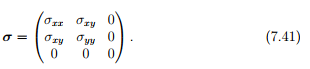
Next, we specialize the above stress formulation for the plane stress case. Without loss of generality, let us assume that the Cartesian components of this plane stress state is
Further, let us assume that body forces are absent and that the Airy’s stress function depends on only x and y. Thus, β = 0 and  Note that this assumption for the Airy’s stress function does not ensure σzz = 0, whenever
 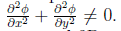 . Hence, plane stress formulation is not a specialization of the general 3D problem. Therefore, we have to derive the governing equations again following the same procedure.
Since, we assume that there are no body forces and the Airy’s stress function depends only on x and y, the Cartesian components of the stress are related to the Airy’s stress function as,
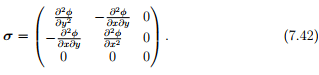
Substituting for stress from equation (7.42) in the constitutive relation (7.4) we obtain,
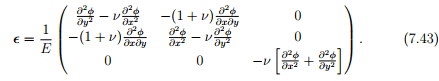
Substituting for strain from equation (7.43) in the compatibility condition (7.7) through (7.12), the non-trivial equations are
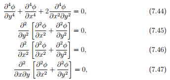
Now, for equations (7.45) through (7.47) to hold,
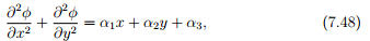
where αi ’s are constants. Differentiating equation (7.48) with respect to x twice and adding to this the result of differentiation of equation (7.48) with respect to y twice, we obtain equation (7.44). Thus, for equations (7.44) through (7.47) to hold it suffices that φ satisfy equation (7.48) along with the prescribed boundary conditions. Comparing the expression for €zz in equation (7.43) and the requirement (7.48) arising from compatibility equations (7.8), (7.9) and (7.11) is a restriction on how the out of plane normal strain can vary, i.e.,€zz = ¯α1x + ¯α2y + ¯α3, where ¯αi ’s are some constants. Hence, this requirement that φ satisfy equation (7.48) does not lead to solution of a variety of boundary value problems. Due to Poisson’s effect plane stress does not lead to plane strain and vice versa, resulting in the present difficulty. To overcome this difficulty, it has been suggested that for plane problems one should use the 2 dimensional constitutive relations, instead of 3 dimensional constitutive relations that we have been using till now.
Since, the constitutive relation is 2 dimensional, plane stress implies plane strain and the three independent Cartesian components of the plane stress and strain are related as,
Inverting the above equations we obtain
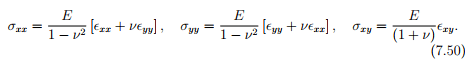
By virtue of using (7.49) to compute the strain for the plane state of stress given in equation (7.42), the only non-trivial restriction from compatibility condition is (7.7) which requires that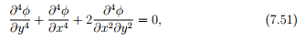
Equation (7.51) is called as the bi-harmonic equation. Thus, for two dimensional problems formulated using stress, one has to find the Airy’s stress potential that satisfies the boundary conditions and the bi-harmonic equation (7.51). Then using this stress potential, the stresses are computed using (7.42). Having estimated the stress, the strain are found from the two dimensional constitutive relation (7.49). Finally, using this estimated strain, the strain displacement relation (7.1) is integrated to obtain the smooth displacement field. We study bending problems in chapter 8 using this approach.
Recognize that equation (7.51) is nothing but ∆(∆(φ)) = 0, where ∆(·) is the Laplacian operator.
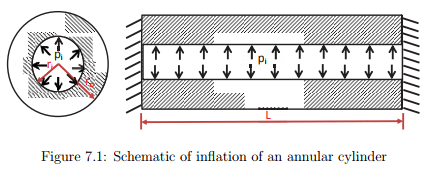
Next, we would like to formulate the plane stress problem in cylindrical polar coordinates. Let us assume that the cylindrical polar components of this plane stress state is
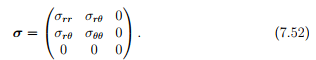
Further, let us assume that body forces are absent and that the Airy’s stress function depends on only r and θ, i.e. φ = φˆ(r, θ). For this case, the Cauchy stress cylindrical polar components are assumed to be
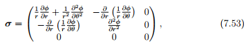
so that it satisfies the static equilibrium equations in the absence of body forces, equation (7.6). Then, using a 2 dimensional constitutive relation, the cylindrical polar components of the strain are related to the cylindrical polar components of the stress through,

As shown before, the only non-trivial restriction from compatibility condition in 2 dimensions is (7.7) and this in cylindrical polar coordinates takes the form,
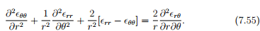
Substituting equation (7.54) and (7.53) in (7.55) and simplifying we obtain,
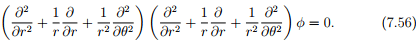
A general periodic solution to the bi-harmonic equation in cylindrical polar coordinates, (7.56) is
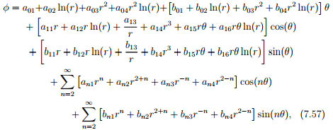
where anm and bnm are constants to be determined from boundary conditions.are constants to be determined from boundary conditions.
FAQs on Techniques to Solve Boundary Value Problems - Civil Engineering (CE)
| 1. What are the key techniques used to solve boundary value problems? |  |
| 2. How does the shooting method work for solving boundary value problems? | |
| 3. What is the finite difference method and how is it used to solve boundary value problems? | |
| 4. How does the finite element method work for solving boundary value problems? | |
| 5. What are spectral methods and how are they used to solve boundary value problems? | |


Techniques to Solve Boundary Value Problems - Civil Engineering (CE)
,past year papers
,video lectures
,Semester Notes
,ppt
,mock tests for examination
,MCQs
,Summary
,Techniques to Solve Boundary Value Problems - Civil Engineering (CE)
,Objective type Questions
,shortcuts and tricks
,Free
,Viva Questions
,Sample Paper
,study material
,Important questions
,practice quizzes
,Techniques to Solve Boundary Value Problems - Civil Engineering (CE)
,Extra Questions
,Previous Year Questions with Solutions
,Exam
;


Techniques to Solve Boundary Value Problems Free PDF Download
Importance of Techniques to Solve Boundary Value Problems
Techniques to Solve Boundary Value Problems Notes
Techniques to Solve Boundary Value Problems Civil Engineering (CE) Questions
Study Techniques to Solve Boundary Value Problems on the App
|
© EduRev
|
Education Revolution
|


|


within 7 days!