ICAI Notes: Theoretical Distribution- 2 | Quantitative Aptitude for CA Foundation PDF Download
Applications of Normal Distribution
The applications of normal distribution is not restricted to statistics only. Many science subjects, social science subjects, management, commerce etc. find many applications of normal distributions. Most of the continuous variables like height, weight, wage, profit etc. follow normal distribution. If the variable under study does not follow normal distribution, a simple transformation of the variable, in many a case, would lead to the normal distribution of the changed variable. When n, the number of trials of a binomial distribution, is large and p, the probability of a success, is moderate i.e. neither too large nor too small then the binomial distribution, also, tends to normal distribution. Poisson distribution, also for large value of m approaches normal distribution. Such transformations become necessary as it is easier to compute probabilities under the assumption of a normal distribution. Not only the distribution of discrete random variable, the probability distributions of t, chi-square and F also tend to normal distribution under certain specific conditions. In order to infer about the unknown universe, we take recourse to sampling and inferences regarding the universe is made possible only on the basis of normality assumption. Also the distributions of many a sample statistic approach normal distribution for large sample size.
Example: For a random variable x, the probability density function is given by
Identify the distribution and find its mean and variance.
Solution: The given probability density function may be written as

Thus the given probability density function is that of a normal distribution with μ = 4 and variance = ½.
Example: If the two quartiles of a normal distribution are 47.30 and 52.70 respectively, what is the mode of the distribution? Also find the mean deviation about median of this distribution.
Solution: The 1st and 3rd quartiles of N (μ , σ2) are given by (μ – 0.675 σ) and (μ + 0.675 σ) respectively. As given,
μ – 0.675 σ = 47.30 …. (1)
μ + 0.675 σ = 52.70 …. (2)
Adding these two equations, we get
2 μ = 100 or μ = 50
Thus Mode = Median = Mean = 50. Also σ = 4.
Also Mean deviation about median
= mean deviation about mode
= mean deviation about mean
≅ 0.80σ
= 3.20
Example: Find the points of inflexion of the normal curve
Solution: Comparing f (x) to the probability densities function of a normal variable x , we find that μ = 10 and σ = 4.
The points of inflexion are given by
μ – σ and μ + σ
i.e. 10 – 4 and 10 + 4
i.e. 6 and 13.
Example 17.23: If x is a standard normal variable such that
P (0 ≤ x ≤ b) = a, what is the value of P (|x|≥ b)?
Solution: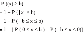

Example: X follows normal distribution with mean as 50 and variance as 100. What is
P(x ≥ 60)? Given ≤ ( 1 ) = 0.8413
Solution: We are given that x ~ N ( μ, σ2 ) where
μ = 50 and σ2 = 100 = > σ = 10
Thus P ( x ≥ 60 )

Example: If a random variable x follows normal distribution with mean as 120 and standard deviation as 40, what is the probability that P (x ≤ 150 / x > 120)? Given that the area of the normal curve between 
Solution: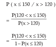
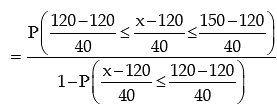
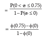

≅0.55
(ϕ ( 0.75) = Area of the normal curve between  = – ∞ to
  = 0.75
= area between – ∞ to 0 + Area between 0 to 0.75 = 0.50 + 0.2734
= 0.7734 )
Example: X is a normal variable with mean = 25 and SD 10. Find the value of b such that
the probability of the interval [2 5, b] is 0.4772 given ϕ (2) = 0.9772.
Solution: We are given that x ~ N ( μ, σ2 ) where μ = 25 and σ = 10
and P [ 25 < x < b ] = 0.4772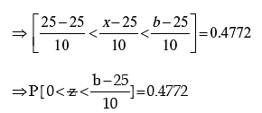

 (as given)
Example: In a sample of 500 workers of a factory, the mean wage and SD of wages are found to be ₹ 500 and ₹ 48 respectively. Find the number of workers having wages:
(i) more than ₹ 600
(ii) less than ₹ 450
(iii) between ₹ 548 and ₹ 600.
Solution: Let X denote the wage of the workers in the factory. We assume that X is normally distributed with mean wage as ₹ 500 and standard deviation of wages as ₹ 48 respectively.
(i) Probability that a worker selected at random would have wage more than ₹ 600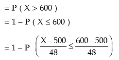
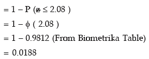
Thus the number of workers having wages less than ₹ 600
= 500 × 0.0188
= 9.4
≅ 9
(ii) Probability of a worker having wage less than ₹450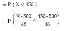

= 1 – 0.8508 (from Biometrika Table)
= 0.1492
Hence the number of workers having wages less than ₹ 450
= 500 × 0.1492
≅ 75
(iii) Probability of a worker having wage between ₹548 and ₹ 600

= 0.9812 – 0.8413 (consulting Biometrika)
= 0.1399
So the number of workers with wages between ₹ 548 and ₹ 600
= 500 × 0.1399
≅ 70.
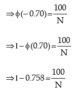
Example: The distribution of wages of a group of workers is known to be normal with mean ₹500 and SD ₹100. If the wages of 100 workers in the group are less than ₹430, what is the total number of workers in the group?
Solution: Let X denote the wage. It is given that X is normally distributed with mean as ₹500 and SD as ₹100 and P (X < 430) = 100/N, N being the total no. of workers in the group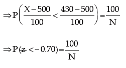

Example: The mean height of 2000 students at a certain college is 165 cms and SD 9 cms. What is the probability that in a group of 5 students of that college, 3 or more students would have height more than 174 cm?
Solution: Let X denote the height of the students of the college. We assume that X is normally distributed with mean (σ) 165 cms and SD (μ) as 9 cms. If p denotes the probability that a student selected at random would have height more than 174 cms., then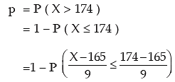
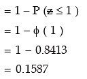
If y denotes the number of students having height more than 174 cm. in a group of 5 students then y ~ β (n, p) where n = 5 and p = 0.1587. Thus the probability that 3 or more students would be more than 174 cm.

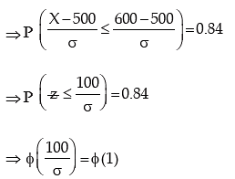
Example: The mean of a normal distribution is 500 and 16 per cent of the values are greater than 600. What is the standard deviation of the distribution? (Given that the area between 
Solution: Let σ denote the standard deviation of the distribution.
We are given that

Example: In a business, it is assumed that the average daily sales expressed in Rupees follows normal distribution. Find the coefficient of variation of sales given that the probability that the average daily sales is less than ₹124 is 0.0287 and the probability that the average daily sales is more than ₹270 is 0.4599.
Solution: Let us denote the average daily sales by x and the mean and SD of x by μ and σ respectively. As given,
From (1), we have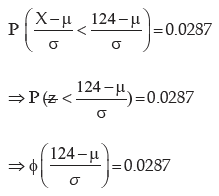
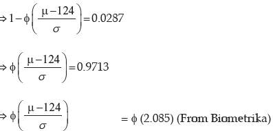
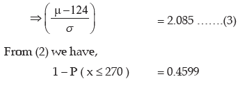
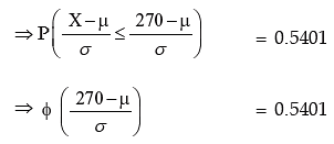
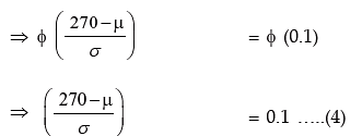
Dividing (3) by (4), we get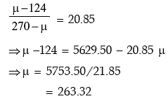
Substituting this value of μ in (3), we get
Thus the coefficient of variation of sales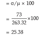
Example: x and y are independent normal variables with mean 100 and 80 respectively and standard deviation as 4 and 3 respectively. What is the distribution of (x + y)?
Solution: We know that if x ~ N (μ1 , σ12 ) and y~ N (μ2 , σ22 ) and they are independent, then z = x + y follows normal with mean (μ1 + μ2 ) and
Thus the distribution of (x + y) is normal with mean (100 + 80) or 180
Standard Normal Distribution: If a continuous random variable z follows standard normal distribution, to be denoted by  N(0, 1), then the probability density function of
  is given by

Some important properties of  are listed below :(i) z has mean, median and mode all equal to zero.
(ii) The standard deviation of  is 1. Also the approximate values of mean deviation and quartile deviation are 0.8 and 0.675 respectively.
(iii) The standard normal distribution is symmetrical about  = 0.
= 0.
(iv) The two points of inflexion of the probability curve of the standard normal distribution are –1 and 1.
(v) The two tails of the standard normal curve never touch the horizontal axis.
(vi) The upper and lower p per cent points of the standard normal variable z are given by
(since for a standard normal distribution 
Selecting P = 0.005, 0.025, 0.01 and 0.05 respectively,
We have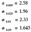
(vii) If  denotes the arithmetic mean of a random sample of size n drawn from a normal population then,
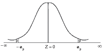
Showing upper and lower p % points of the standard normal variable.
|
148 videos|174 docs|99 tests
|
FAQs on ICAI Notes: Theoretical Distribution- 2 - Quantitative Aptitude for CA Foundation
| 1. What is a theoretical distribution? |  |
| 2. How is a theoretical distribution different from an empirical distribution? |  |
| 3. What are some examples of theoretical distributions? |  |
| 4. How are theoretical distributions used in statistics? |  |
| 5. Can the theoretical distribution perfectly represent real-world data? |  |
|
148 videos|174 docs|99 tests
|

|
Explore Courses for CA Foundation exam
|

|


