Use SUMPRODUCT to Calculate Weighted Averages | How to become an Expert of MS Excel - Class 6 PDF Download

Introduction

Although Excel doesn't have a weighted average function, it does have a function that does most of the work for you: SUMPRODUCT. Even if you've never used SUMPRODUCT before, you'll be able to use it like a pro by the end of this article. The method we're using works with all versions of Excel, and it also works with other spreadsheet applications like Google Sheets.

Setting up the spreadsheet

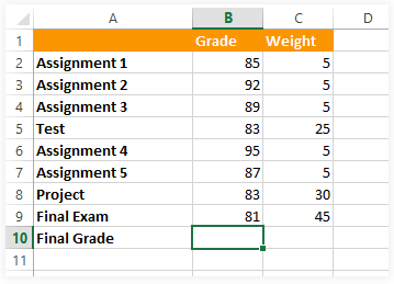
• In order to calculate the weighted average, you'll need at least two columns. The first column (column B in our example) contains the grades for each assignment or test. The second column (column C) contains the weights. A higher weight will cause the assignment or test to have a greater effect on the final grade.

• You can think of the weight as being the percentage of the final grade. But in this case, the weights actually add up to more than 100%. That's OK because our formula will still work no matter what the weights add up to.
  

Entering the formula

• The first part of our formula will be the SUMPRODUCT function. Because the arguments will be in parentheses, go ahead and type an open parenthesis:
  =SUMPRODUCT(
• Next, we'll add the arguments to the function. SUMPRODUCT can have any number of arguments, but it will usually have two. In our example, the first argument will be the cell range B2:B9—the cells that contain our grades:
  =SUMPRODUCT(B2:B9
• The second argument will be the cell range C2:C9—the cells that contain the weights. You'll need to use a comma to separate these two arguments. When you're done, type a closed parenthesis:
  =SUMPRODUCT(B2:B9, C2:C9)
• Now we'll add the second part of our formula. This part will divide SUMPRODUCT by the SUM of the weights. Later, we'll talk about why this is important.
  Start by typing a / (forward slash) for division, and then type the SUM function:
  =SUMPRODUCT(B2:B9, C2:C9)/SUM(
• We just need one argument for the SUM function: the cell range C2:C9. Remember to close the parentheses after the argument:
  =SUMPRODUCT(B2:B9, C2:C9)/SUM(C2:C9)

That's it! When you press Enter on your keyboard, Excel will calculate the weighted average. In our example, the final grade is 83.6.

How it works

• If you're wondering why the values needed to be multiplied in the first place, think of it this way: The assignments with a higher weight are counted more times. For example, Assignment 2 is counted 5 times, but the Final Exam is counted 45 times. This is why the Final Exam has a bigger impact on the final grade. By comparison, a "regular" average would count each assignment one time, so each one has the same weight.
• If you could look "under the hood" of the SUMPRODUCT function, you would see that this is what it is actually calculating:
  =(B2*C2)+(B3*C3)+(B4*C4)+(B5*C5)+(B6*C6)+(B7*C7)+(B8*C8)+(B9*C9)
• Luckily, we don't have to write a long formula like this because SUMPRODUCT is doing all of it automatically.
• By itself, SUMPRODUCT will give us a huge number: 10,450. This is where the second part of our formula comes in: /SUM(C2:C9). This part brings the value back down to a normal grade range, making the answer 83.6.

The second part of the formula is actually really useful because it allows the formula to automatically correct its calculations. Remember that the weights don't need to add up to 100%? This is because this part of the formula takes care of that for us. For example, if we increase one or more of the weights, the second part of the formula simply divides by a higher number, bringing it back down to the correct answer. We could even make the weights much smaller, giving them values like 0.5, 2.5, 3.0, and 4.5, and the formula would still work perfectly.