Introduction to Signal & Systems


Introduction
The intent of this introduction is to give the reader an idea about signals and systems as a field of study and their applications. Before proceeding further, we give clear, working definitions of the two fundamental ideas.
Basic definitions
- Signal: A signal is a function of one or more independent variables that conveys information. Common independent variables are time and space. Signals are often written as x(t) for continuous-time signals or x[n] for discrete-time signals.
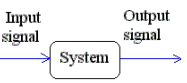
- System: A system is any physical or conceptual device or process that accepts one or more input signals and produces one or more output signals. A system describes a relationship (or mapping) from input(s) to output(s).
Examples of signals
- Voltage signal: Voltage across two points as a function of time, v(t).
- Force pattern: Force defined as a function of two-dimensional space, F(x,y), for example pressure distribution on a plate.
- Photograph: Intensity and colour as functions of two spatial variables, I(x,y).
- Video signal: A sequence of images - intensity and colour as functions of two spatial variables and time, I(x,y,t).
Examples of systems
- Oscilloscope: Accepts an electrical voltage and produces a two-dimensional visual trace representing voltage versus time.
- Computer monitor: Receives digital/analog signals from a graphics system and produces a time-varying visual display.
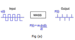
- Accelerating mass (mechanical system): An applied force f(t) can be regarded as an input and the resulting velocity v(t) or displacement x(t) as the output.
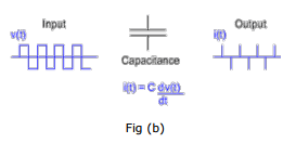
- Capacitor (electrical system): The terminal voltage v(t) and current i(t) are related by i(t)=C dv(t)/dt, so one may treat voltage as input and current as output or vice versa depending on the analysis.
Mechanical and electrical examples
You will have studied many of these systems in separate courses (mechanics, electrostatics, circuits). In signals and systems we develop general methods that are independent of the physical origin. Thus, the same mathematical tools apply to electrical, mechanical, chemical or biological systems when they are described by input-output relationships.
Why study signals and systems?
Studying signals and systems provides tools to:
- Characterise signals and systems - describe behaviour quantitatively.
- Design systems that have desired properties for processing, filtering or controlling signals.
- Modify existing systems to improve performance, stability, response or robustness.
The focus is on the relationship between input and output signals rather than internal implementation details. Once input-output behaviour is known, the results apply across contexts.
Classification of signals
- Continuous-time vs discrete-time: A continuous-time signal x(t) is defined for all real t. A discrete-time signal x[n] is defined only at integer indices n.
- Analog vs digital: An analog signal has a continuum of amplitude values. A digital signal has discrete amplitude levels (often after quantisation).
- Periodic vs aperiodic: A signal x(t) is periodic if x(t+T)=x(t) for some T>0. If no such T exists, it is aperiodic.
- Even and odd: A signal is even if x(-t)=x(t) and odd if x(-t)=-x(t). Signals can be decomposed into even and odd parts.
- Deterministic vs random (stochastic): Deterministic signals are exactly specified by a formula; random signals are described statistically.
- Energy and power signals: Energy of a continuous-time signal is E = ∫_{-∞}^{∞} |x(t)|^2 dt and the average power is P = lim_{T→∞} (1/2T) ∫_{-T}^{T} |x(t)|^2 dt. A signal is an energy signal if 0<><∞ and="" power="" is="" zero;="" a="" power="" signal="" has="" finite="" nonzero="" average="" power="" and="" infinite="">
Basic signal operations
- Scaling in amplitude: y(t)=a x(t), a is a constant.
- Time-scaling: y(t)=x(a t), which compresses or expands the signal in time for |a|>1 or |a|<1>
- Time-shifting: y(t)=x(t-t0); the signal is delayed by t0 if t0>0, or advanced if t0<>
- Time-reversal: y(t)=x(-t), mirror image about t=0.
- Addition and multiplication: Superposition y(t)=x1(t)+x2(t) and modulation y(t)=x1(t)·x2(t).
Classification and properties of systems
- Linearity: A system is linear if it satisfies superposition: if x1→y1 and x2→y2 then ax1+bx2→ay1+by2 for constants a,b.
- Time-invariance: A system is time-invariant if a delay in the input produces an identical delay in the output. If x(t-t0) produces y(t-t0) for every t0, the system is time-invariant.
- Causality: A causal system does not depend on future values of the input; the output at time t depends only on input values at times ≤t.
- Stability (BIBO stability): A system is BIBO stable if every bounded input produces a bounded output. That is, if |x(t)|≤Mx<∞ for="" all="" t="" then=""><∞ for="" all="">
- Memoryless vs with memory: A memoryless system's output at time t depends only on the input at the same time t. Otherwise it has memory.
- Invertibility: A system is invertible if distinct inputs produce distinct outputs and there exists an inverse system that recovers the input from the output.
- Realizability: A physically realisable system must respect causality and typically be implementable with available components.
Linear Time-Invariant (LTI) systems
LTI systems are central because they combine linearity and time-invariance. For LTI systems the output is determined completely by the impulse response h of the system, and the input x by convolution with h.
- Continuous-time convolution: y(t)=∫_{-∞}^{∞} x(τ) h(t-τ) dτ.
- Discrete-time convolution: y[n]=∑_{k=-∞}^{∞} x[k] h[n-k].
- The impulse response h(t) is the output when the input is the Dirac delta δ(t) (or δ[n] for discrete time). Knowledge of h allows prediction of output for any input using convolution.
Simple analysis remarks
Many general properties follow directly for LTI systems. For example, stability and causality can be determined from h(t):
- If h(t)=0 for t<0 the="" system="" is="">
- If ∫_{-∞}^{∞} |h(t)| dt < ∞="" the="" system="" is="" bibo="" stable="" (continuous="" time);="" an="" analogous="" summation="" condition="" applies="" in="" discrete="">
Applications and examples
- Filtering: Removing unwanted spectral components (noise) from signals using designed systems (filters).
- Modulation and demodulation: Transmitting signals over channels and recovering them at the receiver.
- Control systems: Using system models to design controllers that achieve desired response (stability, steady-state error, transient behaviour).
- Image and video processing: Enhancing, compressing and restoring images and videos using signal-processing systems.
- Biomedical signals: Analysing ECG, EEG and other physiological signals for diagnosis and monitoring.
How this course approaches the subject
We will define properties of signals and systems based on real-life examples and then connect these properties to mathematical consequences. These connections are the tools that allow the same analysis methods to be used for a wide variety of systems - electrical, mechanical, chemical or biological - once the input-output relation is known. The emphasis will be on building intuition, mathematical methods (such as convolution, transforms), and practical examples.
Conclusion
In this lecture you have learnt:
- Signals are functions of one or more independent variables (for example, time or space).
- Systems are models that produce output signals in response to input signals.
- Identifying real-life examples as models of signals and systems helps to understand and apply general analysis techniques.
FAQs on Introduction to Signal & Systems
| 1. What is signal processing? |  |
| 2. How are signals classified in signal processing? | |
| 3. What are systems in signal processing? | |
| 4. What is the Fourier transform in signal processing? | |
| 5. How is signal processing applied in real-world applications? | |


|
Explore Courses for Electrical Engineering (EE) exam
|
|

|
Get EduRev Notes directly in your Google search
|
|