Description of Systems | Signals and Systems - Electrical Engineering (EE) PDF Download
| Table of contents |
|
| What is a system? |
|
| Examples of systems |
|
| System description |
|
| The mapping involved in systems |
|
| Properties of Systems |
|

What is a system?
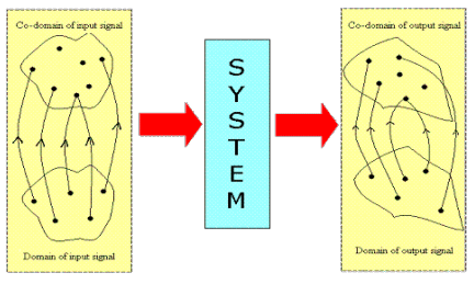
A signal was defined as a mapping from a set of the independent variable (domain) to the set of the dependent variable (co-domain). A system is also a mapping, but across signals, or across mappings . That is, the domain set and the co-domain set for a system are both sets of signals, and corresponding to each signal in the domain set, there exists a unique signal in the co-domain set.
The study of signals and systems concerns two things: information and how that information affects things. A strict definition of a signal is a time-varying occurrence that conveys information, and a strict definition of system is a collection of modules which take in signals and generate some sort of response.
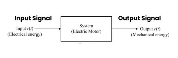
In signals and systems terminology, we say; corresponding to every possible input signal, a system “produces” an output signal.
In that sense, realize that a system, as a mapping is one step hierarchically higher than a signal. While the correspondence for a signal is from one element of one set to a unique element of another, the correspondence for a system is from one whole mapping from a set of mappings to a unique mapping in another set of mappings!
So, a signal function might look like this:
The graph corresponding to this signal would look like this:
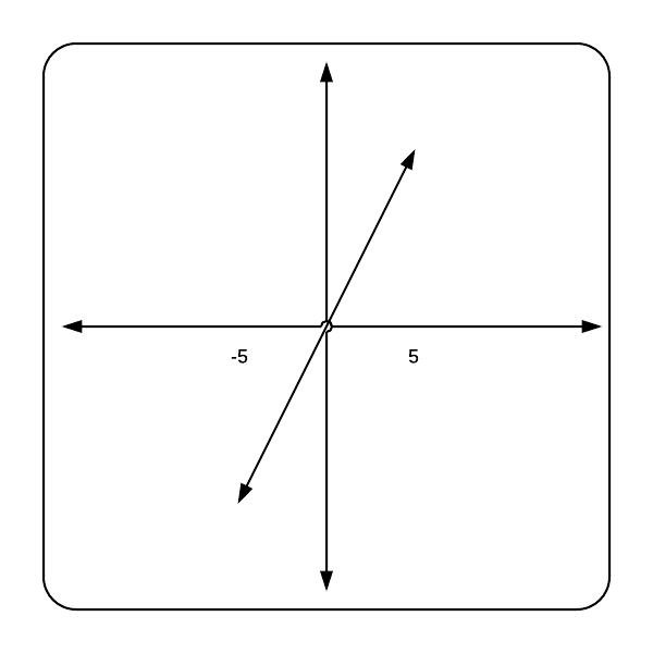 Graph for Signal
A system can have various possible input and output signals.
For instance, consider the example of a robot. The robot might use a camera to detect the color of a line, or it could utilize its tires to physically sense the line if it has distinctive physical properties. Additionally, it could detect magnetic forces if the line is coated with specific materials. While the input signal is usually determined by the surrounding environment, the system has significantly more control over the output signal. The output signal can be any form of information that directs the robot's steering actions.
There are many types of systems and ways to control them. They all have important use cases and applications in the field of systems. There are three ways that systems are generally represented:
- difference equations
- block diagrams
- operator equations.
We will study about those in detail later
Examples of systems
Examples of systems are all around us. The speakers that go with your computer can be looked at as systems whose input is voltage pulses from the CPU and output is music (audio signal). A spring may be looked as a system with the input , say, the longitudinal force on it as a function of time, and output signal being its elongation as a function of time. The independent variable for the input and output signal of a system need not even be the same.
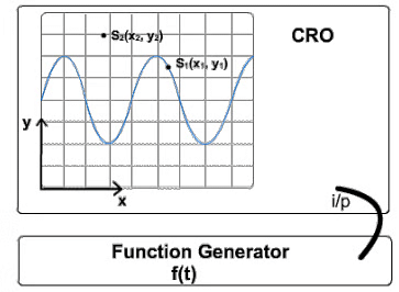
Cathode Ray Oscilloscope
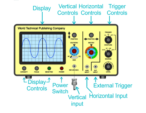
An input voltage signal f(t) is provided to the CRO by using a function generator. The CRO (the system) transforms this input function into an image that is displayed on the CRO screen. The luminosity of every point on this display (i.e. value of the signal) is dependent on the x and y coordinates. So, the output S(x, y) has it's independent variable as space, whereas the input independent variable is time.
In fact, it is even possible for the input signal to be continuous-time and the output signal to be discrete-time or vice-versa. For example, our speech is a continuous-time signal, while a digital recording of it is a discrete-time signal! The system that converts any one to the other is an example of this class of systems.
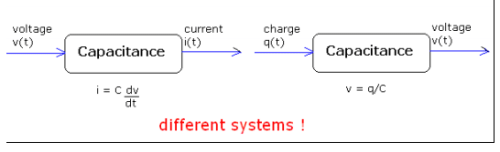
As these examples may have made evident, we look at many physical objects/devices as systems, by identifying some variation associated with them as the input signal and some other variation associated with them as the output signal (the relationship between these, that essentially defines the system depends on the laws or rules that govern the system) . Thus a capacitance with voltage (as a function of time) considered as the input signal and current considered as the output signal is not the same system as a capacitance with, say charge considered as the input signal and voltage considered as the output signal. Why?
The mappings that define the system are different in these two cases.
We shall next discuss what system description means.
System description
The system description specifies the transformation of the input signal to the output signal. In certain cases, a system has a closed form description. E.g. the continuous-time system with description y(t) = x(t) + x(t-1); where x(t) is the input signal and y(t) is the output signal. Not all systems have such a closed form description. Just as certain "pathological" functions can only be specified by tabulating the value of the dependent variable against all values of the independent variable; some systems can only be described by tabulating the output signal against all possible input signals.
Explicit and Implicit Description
When a closed form system description is provided, it may either be classified as an explicit description or an implicit one.
For an explicit description, it is possible to express the output at a point, purely in terms of the input signal. Hence, when the input is known, it is easily possible to find the output of the system, when the system description is Explicit. In case of an Explicit description, it is clear to see the relationship between the input and the output. e.g. y(t) = { x(t) }2 + x(t-5).
In case the system has an Implicit description, it is harder to see the input-output relationship. An example of an Implicit description is y(t) - y(t-1) x(t) = 1. So when the input is provided, we are not directly able to calculate the output at that instant (since, the output at 't-1' also needs to be known). Although in this case also, there are methods to obtain the output based solely on the input, or, to convert this implicit description into an explicit one. The description by itself however is in the implicit form.
The mapping involved in systems
We shall next discuss the idea of mapping in a system in a little more depth.
A signal maps an element in one set to an element in another. A system, on the other hand maps a whole signal in one set to a signal in another. That is why a system is called a mapping over mappings. Therefore, the value of the output signal at any instant of time (remember "time" is merely symbolic) in general depends on the whole input signal. Thus, even if the independent variable for the input and output signal are the same (say time t), do not assume the value the output signal at, say t = 5
depends on only the value of the input signal at t = 5. For example, consider the system with description:
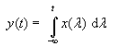
The output at, say t = 5 depends on the values of the input signal for all t <= 5.
Henceforth; we shall call systems with both input and output signal being continuous-time as continuous-time systems , and those with both input and output signal being discrete-time as discrete-time systems. Those that do not fall into either of these classes (i.e. input discrete-time and output continuous-time and vice-versa) we shall call hybrid systems. Now that the necessary introductions are done, we can get on to system properties.
Properties of Systems
Given Below are the Properties of Systems :
- Periodicity
- Even and Odd
- Linearity
- Time Invariant
- LTI Systems
- BIBO
- Stability
- Causality
- Reflection
|
45 videos|70 docs|33 tests
|
FAQs on Description of Systems - Signals and Systems - Electrical Engineering (EE)
| 1. What is a system in the context of this article? |  |
| 2. Can you provide examples of systems mentioned in the article? | |
| 3. How are systems described in the article? | |
| 4. What mapping is involved in systems according to the article? | |
| 5. What are some properties of systems mentioned in the article? | |


Previous Year Questions with Solutions
,past year papers
,Extra Questions
,Description of Systems | Signals and Systems - Electrical Engineering (EE)
,Important questions
,Semester Notes
,Description of Systems | Signals and Systems - Electrical Engineering (EE)
,Objective type Questions
,Sample Paper
,video lectures
,mock tests for examination
,ppt
,Free
,Summary
,shortcuts and tricks
,Exam
,Description of Systems | Signals and Systems - Electrical Engineering (EE)
,Viva Questions
,MCQs
,study material
,practice quizzes
;


Description of Systems Free PDF Download
Importance of Description of Systems
Description of Systems Notes
Description of Systems Electrical Engineering (EE) Questions
Study Description of Systems on the App
|
© EduRev
|
Education Revolution
|


|


within 7 days!