Properties of Fourier Transform

Properties of Fourier Transform
Differentiation and Integration (Time-domain)
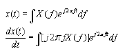
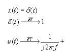
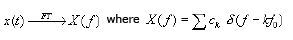
The Fourier transform (FT) of a signal x(t) is defined as X(f) = ∫-∞∞ x(t) e-j2πft dt and the inverse is x(t) = ∫-∞∞ X(f) ej2πft df, where f denotes frequency in Hz. Several useful operations in time correspond to simple algebraic operations in frequency. Below we develop the differentiation and integration properties and explain important caveats (especially at f = 0).
Differentiation in time
If x(t) is differentiable and its derivative is absolutely integrable (so FT exists), the FT of the derivative x'(t) = d/dt x(t) is obtained by differentiating the complex exponential inside the transform integral.
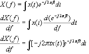
Hence, if X(f) is the Fourier transform of x(t), then
then
Equivalently, using angular frequency ω = 2πf,
Hence if x'(t) exists and FT conditions hold,
then
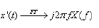
In words: differentiation in time corresponds to multiplication by j2πf (or jω) in frequency:
d/dt x(t) ↔ j2πf X(f) = jω X(ω)
This property is widely used to convert differential equations in time into algebraic equations in frequency.
Integration in time
The inverse operation of time-differentiation is time-integration. Formally, if y(t) = ∫-∞t x(τ) dτ (causal integral) or if Y(f) denotes the FT of an antiderivative of x(t), then the frequency-domain relation involves division by j2πf. Care must be taken about any constant (DC) term introduced by indefinite integration.

Thus, formally,
∫ x(t) dt ↔ X(f) / (j2πf) + C δ(f)
The extra term C δ(f) arises because 1/(j2πf) is singular at f = 0. If x(t) has zero mean (no DC component), the C δ(f) term vanishes and the simple division by j2πf is valid. If x(t) contains a nonzero DC component, the integral grows without bound as t → ∞ and the FT includes an impulse at f = 0 to represent the unbounded or constant component.
Example: consider x(t) = rect(t) (a rectangular pulse). Differentiating x(t) gives impulses at the pulse edges, and the FT of the derivative is j2πf times the FT of rect(t). The integration of the derivative recovers the original pulse up to a constant, and the division by j2πf must account for any DC term.
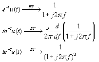
To illustrate the DC/impulse issue, let
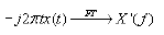
This causes a problem when the spectrum contains a 1/f singularity which produces an impulse in frequency.
The impulse at f = 0 represents the constant (DC) part introduced by indefinite integration.
Scaling of the independent variable
Time-scaling property
If x(t) has Fourier transform X(f), then for a real nonzero constant a the scaled signal x(at) has transform given by a change of variables in the transform integral. The usual form (using frequency f) is:
When a > 0 or a < 0, the transform pair is
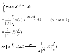
Concretely,
x(at) ↔ (1/|a|) X(f / a)
Thus compression in time (|a| > 1) stretches the spectrum and scales its amplitude by 1/|a|; expansion in time (|a| < 1) compresses the spectrum and increases amplitude by 1/|a|. The amplitude factor ensures preservation of the integral relation between time and frequency representations.
There is also an energy-normalised scaling commonly used in signal processing and physics, where the scaled signal is multiplied by |a|1/2 to preserve total energy:
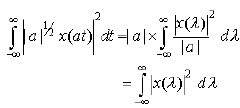
Hence, x(t) and |a|<sup>1/2</sup>x(at) have the same energy. Therefore this scaling is called energy-normalised scaling of the independent variable.
Properties of Fourier Series (periodic signals)
For periodic signals, the Fourier transform becomes a train of impulses at harmonic frequencies and is often expressed via Fourier series (FS) coefficients. Many FT properties have direct analogues in the FS domain. Let x(t) be periodic with period T and fundamental angular frequency ω0 = 2π/T. Its FS expansion is x(t) = Σk=-∞∞ ck ej k ω0 t, where
ck = (1/T) ∫0T x(t) e-j k ω0 t dt
Time-shift
Time shifting a periodic signal multiplies each Fourier series coefficient by a complex exponential. If x(t) has FS coefficients ck, then x(t - t0) has coefficients ck e-j k ω0 t0. This corresponds to the FT property of phase rotation for frequency-domain samples.
We know:
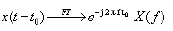
Thus if x(t) is periodic with period T, x(t - t0) has Fourier series coefficients

Differentiation (periodic signals)
If x(t) is differentiable term-by-term (suitable smoothness/decay of coefficients), differentiating x(t) multiplies each FS basis exponential by j k ω0. Hence the FS coefficients of x'(t) are j k ω0 times those of x(t).
If the periodic signal is differentiable then
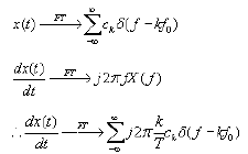
Thus if x(t) is periodic with period T, x'(t) has Fourier series coefficients

In compact form:
d/dt x(t) = Σ j k ω0 ck ej k ω0 t and therefore the kth coefficient of x'(t) is j k ω0 ck.
Scaling of the independent variable (periodic signals)
Scaling a periodic signal in time changes its period. If x(t) has period T, then x(at) has period T/a when a > 0 and period T/(-a) when a < 0. The FS coefficients remain the same numerical sequence ck but now correspond to a different fundamental frequency; the harmonic spacing is multiplied by a.
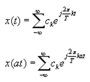
If a > 0, x(at) is periodic with period T/a and the original coefficient ck becomes the Fourier coefficient corresponding to the frequency k(a ω0) = k(2π/(T/a)).

If a < 0, x(at) is periodic with period T/(-a) and the coefficient ck becomes associated with frequency k(a ω0) with sign change as appropriate.

Multiplication by t (time-domain) for a periodic signal
Multiplying a periodic signal by t does not, in general, produce a periodic signal. To analyse this within Fourier series theory, one considers the function defined on one period and then takes its periodic extension. Let x(t) be periodic with period T; define y(t) as t·x(t) on 0 ≤ t < T and extend periodically. The FS coefficients of y(t) relate to the derivative of the coefficients of x(t) with respect to the harmonic index.
Starting from the coefficient definition:
ck = (1/T) ∫0T x(t) e-j k ω0 t dt
and for y(t) = t x(t) (periodically extended), its kth coefficient is
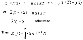
Note the kth Fourier series coefficient of x(t) is

Similarly, let
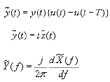
Therefore, the kth Fourier series coefficient of y(t) = t x(t) is

Explicit relationship (obtained by differentiating ck with respect to k and using d/dk e-j k ω0 t = -j ω0 t e-j k ω0 t) is
ck(t x) = j / ω0 · d/dk [ ck ]
This requires that the sequence ck is sufficiently smooth in k so that the derivative with respect to k (treating k as a continuous variable) is meaningful. Without such smoothness (the usual case for arbitrary FS coefficients defined only on integers), this formal relationship needs interpolation or analytic continuation of ck as a function of a continuous index. The idea is not of much practical use without such additional regularity information.

Worked Example
Example:
Consider a simple example where x(t) is a band-limited pulse or a cosine; differentiation and scaling illustrate the above properties.
We show stepwise the effect of differentiation on the FT for an example signal x(t) = cos(2πf0 t):
Take x(t) = cos(2πf0 t).
The Fourier transform of cos(2πf0 t) is X(f) = 0.5 δ(f - f0) + 0.5 δ(f + f0).
Differentiating in time: d/dt x(t) = -2πf0 sin(2πf0 t).
Use the FT differentiation property: FT{d/dt x(t)} = j2πf X(f).
Multiply X(f) by j2πf and evaluate at the impulses: result is j2πf · 0.5 δ(f - f0) + j2πf · 0.5 δ(f + f0).
Using δ(f - f0) picks f = f0 and δ(f + f0) picks f = -f0; the combined spectrum corresponds to the known transform of -2πf0 sin(2πf0 t).
Conclusion
In this chapter you have learned:
- Properties of the Fourier Transform with respect to differentiation and integration, including the important DC/impulse correction for integration.
- Properties of the Fourier Transform with respect to scaling of the independent variable by a real constant a, and the energy-normalised scaling.
- Properties of the Fourier Series with respect to time shifting, and how shifts produce phase rotations of coefficients.
- Properties of the Fourier Series with respect to differentiation, where differentiation in time multiplies each coefficient by j k ω0.
- Properties of the Fourier Series with respect to scaling of the independent variable and the change in fundamental frequency and period.
- Properties of the Fourier Series with respect to multiplication by t, including the relation ck(t x) = j/ω0 · d/dk ck, and the caveat that this requires smoothness (continuous dependence) of the coefficient sequence.
FAQs on Properties of Fourier Transform
| 1. What is the Fourier Transform? |  |
| 2. What are the properties of Fourier Transform? | |
| 3. How does the Fourier Transform help in signal processing? | |
| 4. Can the Fourier Transform be applied to both continuous and discrete signals? | |
| 5. What is the relationship between the Fourier Transform and the Fourier Series? | |


 | Explore Courses for Electrical Engineering (EE) exam |
 | Get EduRev Notes directly in your Google search |